Welcome to MapDork

This site is for “under the hood” details on maps I publish on my substack page. Below is some further detail on my “Kountry” restaurant map.

Interactive map

Code for ggplot2 map

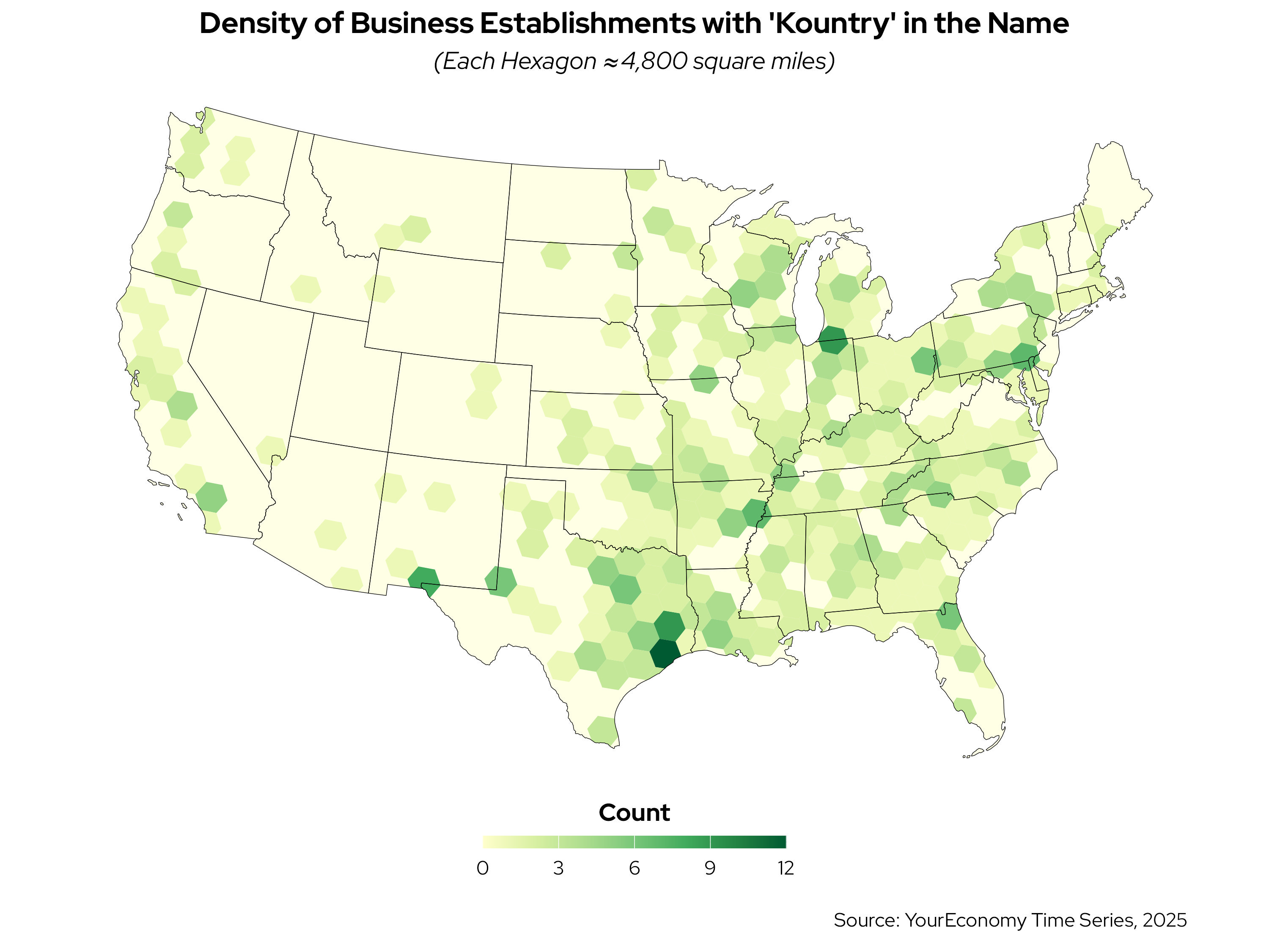
This code aggregates business locations into H3 hexagons at resolution 3 (approximately 4,800 square miles each), counts the number of establishments per hexagon, and clips the results to the contiguous United States. The ggplot2 visualization uses an Albers Equal Area projection and a yellow-green color scale to show the spatial distribution of businesses with “Kountry” in their name.

I use data from the YourEconomy Time Series (YTS), which covers all U.S. business establishments from 1998 to 2025. For legal reasons—i.e., it’s their data, not mine—that data is not provided in this repository.

library(arrow)
library(tidyverse)
library(janitor)
library(sf)
library(h3jsr)
library(tigris)
library(mapgl)

# Contiguous 48 states
states <- states(cb = TRUE, resolution = '20m') |>
  filter(!STUSPS %in% c("AK", "HI") & STATEFP < 60)

ytsdb <- open_dataset('data/yts')
df <- ytsdb |>
  filter(year %in% c(2021:2025), str_detect(tolower(company), 'kountry')) |>
  collect() |>
  filter(state != 'HI' & state != 'AK')

# Clean and prepare spatial data
dsf <- df |>
  mutate(longitude = ifelse(longitude > 0, longitude * -1, longitude)) |>
  st_as_sf(coords = c('longitude', 'latitude'), crs = 4326, remove = FALSE) |>
  st_transform(6350) |> # Transform to Albers
  slice(1, .by = id)

# H3 requires WGS84, so transform back temporarily
dsf <- dsf |>
  mutate(h3_index = point_to_cell(st_transform(geometry, 4326), res = 3))

# Count occurrences per hexagon
hex_counts <- dsf |>
  st_drop_geometry() |>
  count(h3_index, name = "count")

# Convert H3 indices to polygons
hex_sf <- hex_counts |>
  mutate(geometry = cell_to_polygon(h3_index)) |>
  st_as_sf(crs = 4326)

states <- states |> st_transform(6350) |> select(st = STUSPS)
hex_sf <- hex_sf |> st_transform(6350) |> st_intersection(states)

ggplot() +
  geom_sf(data = states, fill = '#FFFFE5', color = NA) +
  geom_sf(data = hex_sf, aes(fill = count), color = NA) +
  geom_sf(data = states, fill = NA, color = "black", linewidth = .15) +
  scale_fill_distiller(
    palette = 'YlGn',
    direction = 1,
    name = 'Count',
    limits = c(0, 12)
  ) +
  theme_void(base_family = 'Red Hat Display', base_size = 14) +
  labs(
    title = "Density of Business Establishments with 'Kountry' in the Name",
    subtitle = '(Each Hexagon ≈ 4,800 square miles)',
    caption = '\nSource: YourEconomy Time Series, 2025    \n'
  ) +
  theme(
    plot.title = element_text(face = "bold", hjust = 0.5),
    plot.subtitle = element_text(face = "italic", hjust = 0.5),
    legend.title = element_text(face = "bold", hjust = 0.5),
    legend.position = 'bottom'
  ) +
  guides(
    fill = guide_colourbar(
      barheight = 0.5,
      barwidth = 12,
      title.position = "top"
    )
  )