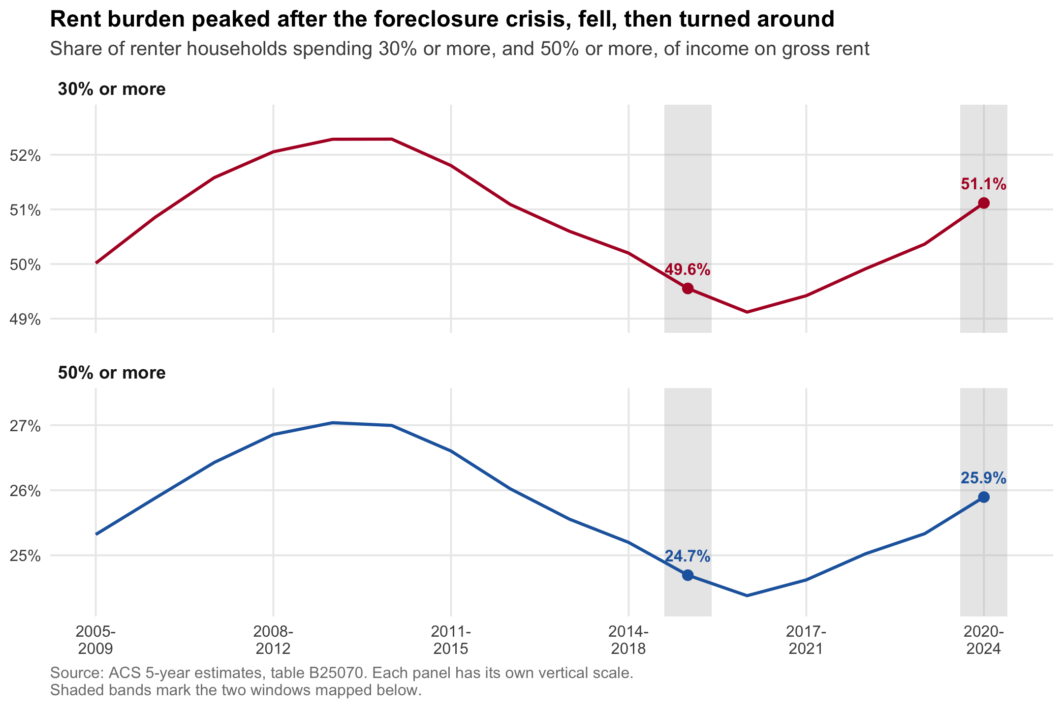
A household is conventionally called rent burdened when gross rent takes up 30 percent or more of household income.1 By that definition, roughly half of American renters are burdened, and the share has been climbing since 2019. This post takes ACS table B25070 at two non-overlapping five-year windows—2015-2019 and 2020-2024—and maps where the increase landed.
One bit of housekeeping before anything else. Writing out both endpoints every time gets unbearable, so from here on a single year is shorthand for the five-year window ending in it: 2019 means the 2015-2019 estimates, 2024 means 2020-2024. That is the Census Bureau’s own labeling and it is how you ask for the files (get_acs(year = 2024) returns 2020-2024). Where the window itself is the point, as in the next section, the full range is spelled out.
The short version: the national share went from 49.6 percent to 51.1 percent, the increase is concentrated in metropolitan counties rather than rural ones, and it is heavily a Sun Belt story. Nevada, Florida, Texas, Arizona and Georgia lead, and in Nevada every single county got worse.
Everything below runs from this one file. The complete script is at the bottom of the post.
The long view
Picking two years a decade apart would have been the obvious move, but it would have been a mistake. Rent burden is not on a trend, it is on a U-shaped curve. Here’s every ACS five-year estimate ever published, from 2005-2009 through to 2020-2024:
The peak sits at 2009-2013 and 2010-2014, right after the foreclosure crisis pushed a wave of former owners into the rental market. The “trough” is 2016-2020. Since then it has risen every single year.
Pulling the data
B25070 breaks renter households into bins by the share of income they spend on gross rent. Anything from _007 up is 30 percent or more. Line _001 is the total, but it includes _011, the households whose ratio could not be computed (zero or negative income, no cash rent), so that group comes out of the denominator.
Margins of error are carried through the whole calculation, because they turn out to be an important part of the story. Weighting by renter households, the national burdened share went from 49.6% to 51.1%, and the median county moved +0.6 points.
Where it is worst right now
Everything after this section is about change. Before getting there it is worth looking at the level, because the two are not the same map.
Florida is the most rent-burdened state in the country: 60.1% of its renters hand over at least 30 percent of their income, against 51.1 percent nationally. Broward, Miami-Dade and Palm Beach counties all clear 62 percent. Hawaii, Nevada and California come next.
The raw change
The map above is mostly wrong. Those familiar with the ACS will immediately know why.
The ACS is a sample, and in a county with only a few hundred renter households, the margin of error on a five-year change runs past ±18 points. Only 21% of counties have a change a 90 percent confidence interval can tell apart from zero.
Shrinking out the noise
Rather than blanking those counties out, let’s shrink them. Comparing the spread of the estimates against their own margins of error yields an estimate of how much the true county changes actually vary; each county’s estimate is then blended with a prior in proportion to its own precision. A well-measured county keeps its own number, a hopeless one leans almost entirely on the prior, and those in between land somewhere in the middle. Importantly, every county still appears on the map.2
One obvious-seeming choice to remedy this problem is to rely on the county’s state average. However, because this strategy pulls smaller counties’ estimates toward the statewide average, it really just ends up making the state look just like its largest metro (Clark County holds 77 percent of Nevada’s weight, and Maricopa 64 percent of Arizona’s, to give two examples). This can also yield hard discontinuities at state lines, leading keen observers to be immediately distrustful of what they’re looking at.
To get around that issue, we use each county’s neighbors instead, a widely used strategy in disease mapping.3 Going back to our Nevada example, Nye County would borrow from Clark because Pahrump is a true Las Vegas exurb, while Eureka County, three hundred miles to the north, would not.
The between-county standard deviation of the true change comes out to 5.0 points, against an observed spread of 10.4. Roughly 77% of the variation in the first map is sampling noise. Note the narrower scale below.
For the median county, the posterior mean (we’ll call it the shrinkage estimate from here on) draws 40% of its weight from the county’s own data, rising to 87% among the largest counties.
Where it rose
| State | Counties | Renters (000s) | 30%+ | 50%+ | Counties rising |
|---|---|---|---|---|---|
| Nevada | 17 | 455 | +6.1 | +4.6 | 100% |
| Texas | 254 | 3856 | +3.9 | +2.7 | 71% |
| Florida | 67 | 2653 | +3.7 | +2.7 | 91% |
| Arizona | 15 | 870 | +3.6 | +1.6 | 53% |
| South Carolina | 46 | 530 | +3.3 | +2.1 | 67% |
| Georgia | 159 | 1290 | +3.3 | +2.9 | 55% |
| Nebraska | 93 | 248 | +2.5 | +1.7 | 63% |
| Utah | 29 | 317 | +2.5 | +1.3 | 45% |
| Massachusetts | 14 | 986 | +2.3 | +1.6 | 93% |
| Minnesota | 87 | 604 | +2.2 | +1.3 | 64% |
Nevada is the extreme case. No state rose more, and it’s the only one where every county did. Clark County by itself holds 76 percent of Nevada’s renters and moved +6.2 points.
Below the state level the pattern is a roll call of growth-magnet metros. Gwinnett County, Georgia (Atlanta suburbs/exurbs) leads the large counties at +9.6, followed by Seminole and Lee counties in Florida (Orlando & Fort Myers), Tarrant County in Texas (Fort Worth), and Davidson County, Tennessee (Nashville).
Here’s what happens when we sort counties into quintiles by renter households:
| Renters in county | Total renters | Change in 30%+ share | Counties rising |
|---|---|---|---|
| Smallest fifth (median 323) | 0.2M | +0.1 | 53% |
| Second (982) | 0.6M | −0.9 | 47% |
| Middle (2,116) | 1.4M | 0.0 | 53% |
| Fourth (4,876) | 3.4M | +0.5 | 55% |
| Largest fifth (22,997) | 36.1M | +1.7 | 71% |
The 82 counties with more than 100,000 renter households hold 48 percent of the country’s renters between them, and 83 percent of them got worse. Rural America is roughly where it was in 2019, while the places where most people actually rent are not.
This is about what supply and demand would predict. Demand has been arriving in Las Vegas, the Dallas suburbs and Central Florida, and rents went with it. The places people have been moving to are the places where rent gets bid up. The rural end is where intuition tends to mislead us. Just because rural places are typically associated with higher poverty rates and lower incomes doesn’t mean the housing affordability crisis of recent years would automatically hit them the hardest. Rents there are lower to begin with, and they have not been bid up the same way.
Moving the Threshold
A fair objection to all of this is that 30 percent is an arbitrary line. A household at 29 percent and one at 31 percent are not meaningfully different, and if the increase were really just households drifting across that boundary, then tightening the definition should make most of it disappear.
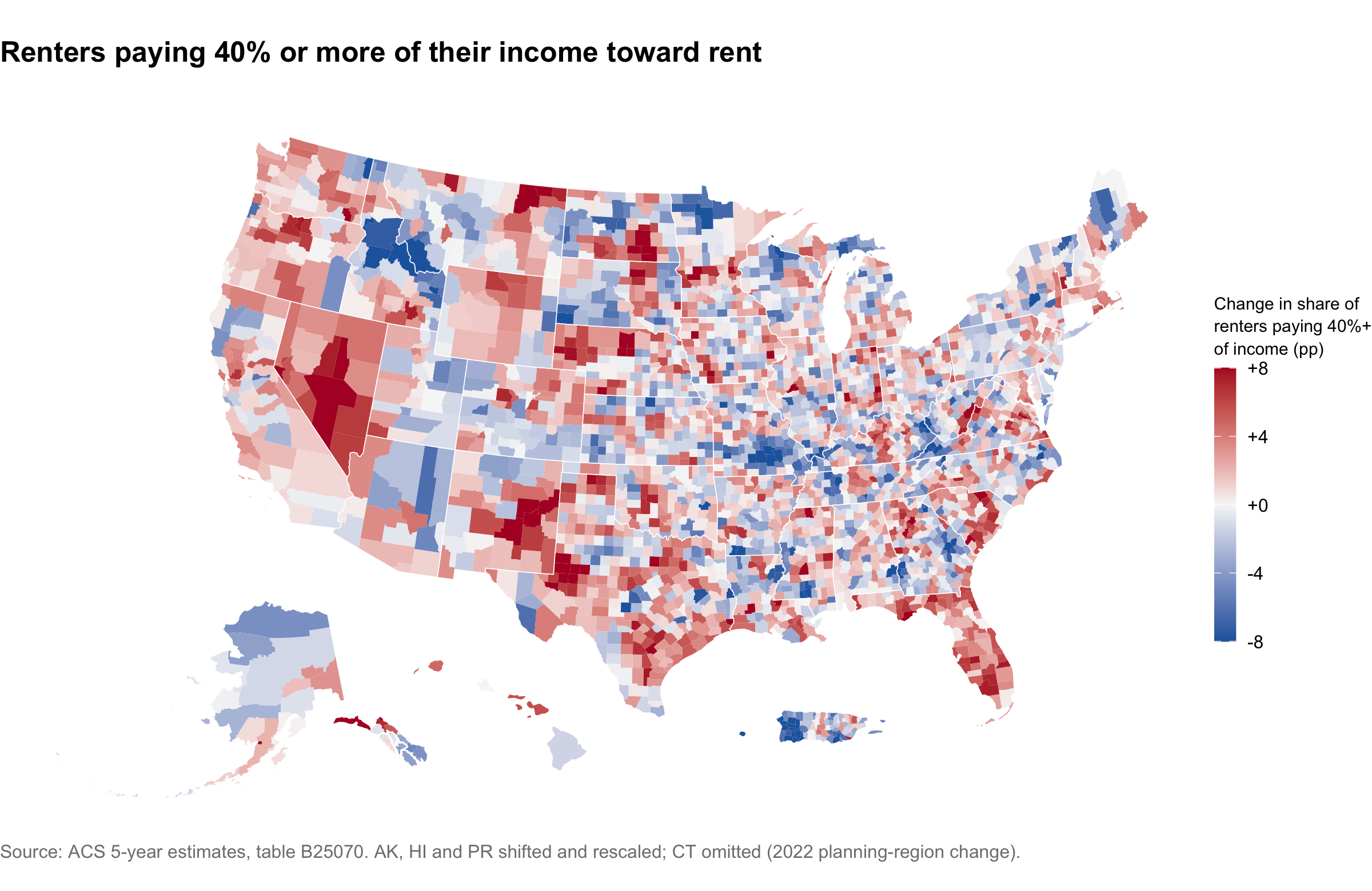
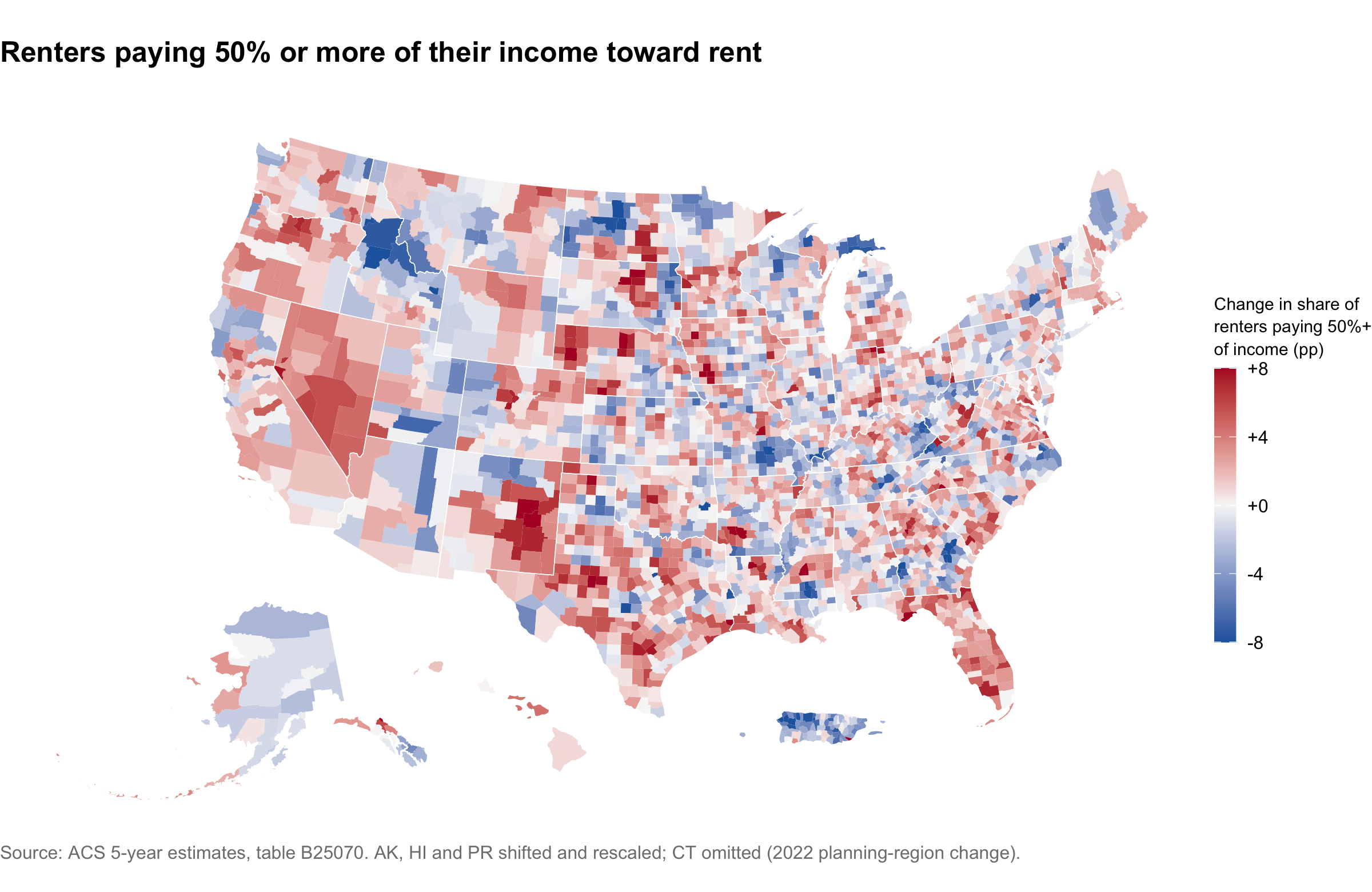
So what happens if we move the threshold for what it means to be “rent-burdened”? The two maps below repeat the shrinkage estimates at stricter cuts, first for renters paying 40 percent or more of their income and then for those paying 50 percent or more. Same window, same neighbor shrinkage, and the same color scale as before, so all three can be read against each other directly.
Concluding Thoughts
While I do have a few papers that focus on housing, I wouldn’t really consider myself a housing researcher. Truly, I only decided to make this map because I was fiddling around with data.census.gov while writing a problem set for my data science class…I saw the rent burden variable and thought, ‘Hmmm, that might make for an interesting map!’
And yet, even for someone without housing policy chops such as myself, there are a few things here that are worth pointing out.
The answer depends almost entirely on which year you start from. Run this same analysis from 2014 and you get -1.2 points, and you would write a post about rent burden easing. Run it from 2019 and you get +1.5 points. Neither number is wrong. The first one just happens to start at the worst moment in modern rental affordability and is therefore measuring a recovery from the foreclosure crisis, not anything about the last five years. This is the sort of thing that makes me nervous about any chart with two endpoints and nothing in between.
Where people moved is where rent got worse. The increases are not spread evenly, and they are not in the places that get written about as expensive. They are in Las Vegas, in the Atlanta and Dallas suburbs, in Nashville, and across most of Florida. These are the destinations of the past five years, and the rental stock does not appear to have kept up.
This is now a metropolitan problem. The largest fifth of counties, holding 86 percent of American renters, rose +1.7 points. Rural counties went essentially nowhere. Whatever national average you quote is really a statement about big metros.
It is not an artifact of the 30 percent line. If households were merely drifting from just under the threshold to just over it, the stricter cuts would barely move. They move nearly as much: the 40 percent share is up 1.3 points and the 50 percent share up 1.2. More renters are severely burdened than five years ago, which is the number I think matters.
So the rhetoric about rent being unaffordable is not wrong. It just does not describe the whole country evenly, and it describes the last five years far better than it describes the last ten.
Source. ACS 5-year estimates, table B25070, via tidycensus. Geometry from tigris at 20m generalized resolution.
Data
NoteFull script
# ---- setup ---------------------------------------------------------
library(tidyverse)
library(tidycensus)
library(tigris)
library(sf)
library(spdep)
library(scales)
library(mapgl)
library(glue)
options(tigris_use_cache = TRUE)
VARS <- c("B25070_001", "B25070_007", "B25070_008",
"B25070_009", "B25070_010", "B25070_011")
# ---- series --------------------------------------------------------
# National totals for every five-year vintage. Cheap: one row per year.
series <- map(2009:2024, \(y) {
get_acs("us", VARS, year = y, survey = "acs5", output = "wide", cache_table = TRUE) |>
rename_with(\(x) str_replace(x, "^B25070_", "v"), starts_with("B25070_")) |>
transmute(
end = y,
renters = v001E - v011E,
`30% or more` = 100 * (v007E + v008E + v009E + v010E) / renters,
`50% or more` = 100 * v010E / renters
)
}) |>
list_rbind() |>
pivot_longer(c(`30% or more`, `50% or more`),
names_to = "threshold", values_to = "pct")
ends <- filter(series, end %in% c(2019, 2024))
# Each threshold gets its own y scale. On a shared axis the 3-point swing in a
# 50-point range reads as a flat line, which is exactly what the chart is
# meant to argue against.
ggplot(series, aes(end, pct, color = threshold)) +
annotate("rect", xmin = 2018.6, xmax = 2019.4, ymin = -Inf, ymax = Inf,
fill = "grey70", alpha = 0.3) +
annotate("rect", xmin = 2023.6, xmax = 2024.4, ymin = -Inf, ymax = Inf,
fill = "grey70", alpha = 0.3) +
geom_line(linewidth = 0.9) +
geom_point(data = ends, size = 2.6) +
geom_text(data = ends, aes(label = sprintf("%.1f%%", pct)),
vjust = -1.2, size = 3.5, fontface = "bold", show.legend = FALSE) +
facet_wrap(~threshold, ncol = 1, scales = "free_y") +
scale_color_manual(values = c("30% or more" = "#b2182b", "50% or more" = "#2166ac")) +
scale_x_continuous(breaks = seq(2009, 2024, 3),
labels = \(x) paste0(x - 4, "-\n", x)) +
scale_y_continuous(labels = \(x) paste0(x, "%"),
expand = expansion(mult = c(0.12, 0.2))) +
labs(
title = "Rent burden peaked after the foreclosure crisis, fell, then turned around",
subtitle = "Share of renter households spending 30% or more, and 50% or more, of income on gross rent",
x = NULL, y = NULL,
caption = "Source: ACS 5-year estimates, table B25070. Each panel has its own vertical scale.\nShaded bands mark the two windows mapped below."
) +
theme_minimal(base_size = 12) +
theme(
legend.position = "none",
strip.text = element_text(face = "bold", hjust = 0, size = 11),
panel.grid.minor = element_blank(),
panel.spacing.y = unit(14, "pt"),
plot.title = element_text(face = "bold", size = 14),
plot.subtitle = element_text(color = "grey30", margin = margin(b = 8)),
plot.caption = element_text(color = "grey50", hjust = 0),
plot.background = element_rect(fill = "white", color = NA)
)
# ---- pull-acs ------------------------------------------------------
# Standard Census formulas for derived estimates: root-sum-square for sums and differences, and the proportion formula for a share. Written out so they stay vectorized over the whole data frame.
moe_rss <- function(...) sqrt(rowSums(cbind(...)^2))
moe_share <- function(num, den, m_num, m_den) {
p <- num / den
under <- m_num^2 - (p^2 * m_den^2)
# Negative radicand: fall back to the ratio formula, per Census guidance
sqrt(ifelse(under < 0, m_num^2 + (p^2 * m_den^2), under)) / den
}
pull_burden <- function(year, geometry = FALSE) {
get_acs(
geography = "county", variables = VARS, year = year, survey = "acs5",
output = "wide", geometry = geometry,
resolution = "20m", # generalized boundaries: ~50x smaller, plots faster
cache_table = TRUE
) |>
rename_with(\(x) str_replace(x, "^B25070_", "v"), starts_with("B25070_")) |>
mutate(
renters = v001E - v011E,
renters = if_else(renters > 0, renters, NA_real_),
renters_moe = moe_rss(v001M, v011M),
burdened = v007E + v008E + v009E + v010E,
burdened_moe = moe_rss(v007M, v008M, v009M, v010M),
pct = 100 * burdened / renters,
pct_moe = 100 * moe_share(burdened, renters, burdened_moe, renters_moe),
# The same measure at stricter thresholds: 40%+ is bins _009 and _010, 50%+ is _010 on its own.
pct40 = 100 * (v009E + v010E) / renters,
pct40_moe = 100 * moe_share(v009E + v010E, renters, moe_rss(v009M, v010M), renters_moe),
pct50 = 100 * v010E / renters,
pct50_moe = 100 * moe_share(v010E, renters, v010M, renters_moe)
) |>
select(GEOID, NAME, any_of("geometry"), renters, burdened,
pct, pct_moe, pct40, pct40_moe, pct50, pct50_moe)
}
b19 <- pull_burden(2019)
b24 <- pull_burden(2024, geometry = TRUE)
# ---- build-change --------------------------------------------------
burden <- b24 |>
select(GEOID, NAME, renters_24 = renters, burdened_24 = burdened,
pct_24 = pct, pct_24_moe = pct_moe,
pct40_24 = pct40, pct40_24_moe = pct40_moe,
pct50_24 = pct50, pct50_24_moe = pct50_moe) |>
separate_wider_delim(NAME, ", ", names = c("county", "state"),
too_many = "merge") |>
inner_join(
b19 |> select(GEOID, renters_19 = renters, burdened_19 = burdened,
pct_19 = pct, pct_19_moe = pct_moe,
pct40_19 = pct40, pct40_19_moe = pct40_moe,
pct50_19 = pct50, pct50_19_moe = pct50_moe),
by = "GEOID"
) |>
st_as_sf() |>
mutate(
change = pct_24 - pct_19,
change_moe = moe_rss(pct_24_moe, pct_19_moe),
sig = abs(change) > change_moe, # 90% CI excludes zero
change40 = pct40_24 - pct40_19,
change40_moe = moe_rss(pct40_24_moe, pct40_19_moe),
change50 = pct50_24 - pct50_19,
change50_moe = moe_rss(pct50_24_moe, pct50_19_moe)
) |>
filter(!is.na(change)) |>
st_transform(4326) # mapgl wants lon/lat; the ggplot maps get shifted later
# The interactive maps each embed their own copy of the boundaries, so they get a simplified one. ms_simplify works on the shared topology rather than polygon by polygon, so counties still tile with no slivers between them. keep = 0.35 takes about a third off the payload while leaving coastlines like the Mississippi delta still recognisable when a reader zooms in; much lower than that and they visibly polygonise.
geom_ll <- burden |>
select(GEOID) |>
rmapshaper::ms_simplify(keep = 0.35, keep_shapes = TRUE)
# State outlines dissolved from the same simplified boundaries, so the overlay lines up with the county edges exactly.
states_ll <- geom_ll |>
left_join(st_drop_geometry(burden) |> select(GEOID, state), by = "GEOID") |>
group_by(state) |>
summarise(.groups = "drop")
us48 <- states_ll |> filter(!state %in% c("Alaska", "Hawaii", "Puerto Rico"))
# Attaches just the columns a given map needs to the light geometry.
map_sf <- function(...) {
geom_ll |>
left_join(st_drop_geometry(burden) |> transmute(GEOID, ...), by = "GEOID") |>
select(-GEOID)
}
# Diverging ramp matching the static maps further down.
div_pal <- colorRampPalette(c("#2166ac", "#f7f7f7", "#b2182b"))
# ---- map-level -----------------------------------------------------
lvl <- burden |>
st_drop_geometry() |>
group_by(state) |>
summarise(level = weighted.mean(pct_24, renters_24),
chg = weighted.mean(change, renters_24), .groups = "drop")
lvl_sf <- map_sf(
pct_24,
tooltip = glue(
"<b>{county}, {state}</b><br>",
"{sprintf('%.1f', pct_24)}% of renters pay 30%+ of income<br>",
"{comma(round(renters_24))} renter households"
)
)
maplibre(bounds = us48, style = carto_style("positron")) |>
add_source(id = "counties", data = lvl_sf) |>
add_fill_layer(
id = "Rent burden",
source = "counties",
fill_color = interpolate(
column = "pct_24", values = c(35, 50, 65),
stops = RColorBrewer::brewer.pal(3, "YlOrRd"), na_color = "lightgrey"
),
fill_opacity = 0.85,
tooltip = "tooltip"
) |>
add_line_layer(id = "county_outlines", source = "counties",
line_color = "black", line_width = 0.05) |>
add_line_layer(id = "state_outlines", source = states_ll,
line_color = "black", line_width = 0.4) |>
add_continuous_legend(
"Renters paying 30%+ of income, 2024",
values = c("35%", "50%", "65%+"),
colors = RColorBrewer::brewer.pal(3, "YlOrRd"),
position = "bottom-left"
)
# ---- map-helper ----------------------------------------------------
# Both static maps are the same diverging choropleth, differing only in the column they fill by and how wide the scale runs.
burden_map <- function(col, cap, title, subtitle, thresh = 30) {
ggplot(burden_sh) +
geom_sf(aes(fill = .data[[col]]), color = NA) +
geom_sf(data = states_sh, fill = NA, color = "white", linewidth = 0.2) +
scale_fill_gradient2(
low = "#2166ac", mid = "#f7f7f7", high = "#b2182b", midpoint = 0,
limits = c(-cap, cap), oob = scales::squish,
labels = \(x) sprintf("%+g", x),
name = sprintf("Change in share of\nrenters paying %d%%+\nof income (pp)", thresh),
guide = guide_colorbar(barheight = 10, barwidth = 0.8)
) +
labs(title = title, subtitle = subtitle,
caption = "Source: ACS 5-year estimates, table B25070. AK, HI and PR shifted and rescaled; CT omitted (2022 planning-region change).") +
theme_void(base_size = 12) +
theme(
plot.title = element_text(face = "bold", size = 15),
plot.subtitle = element_text(color = "grey30", margin = margin(b = 8)),
plot.caption = element_text(color = "grey50", hjust = 0),
legend.title = element_text(size = 9, lineheight = 1.1),
plot.background = element_rect(fill = "white", color = NA)
)
}
# ---- map-raw -------------------------------------------------------
raw_sf <- map_sf(
change,
tooltip = glue(
"<b>{county}, {state}</b><br>",
"Change since 2019: {sprintf('%+.1f', change)} pp<br>",
"Margin of error: ±{sprintf('%.1f', change_moe)} pp<br>",
"{comma(round(renters_24))} renter households"
)
)
maplibre(bounds = us48, style = carto_style("positron")) |>
add_source(id = "counties", data = raw_sf) |>
add_fill_layer(
id = "Raw change",
source = "counties",
fill_color = interpolate(
column = "change", values = c(-15, 0, 15),
stops = div_pal(3), na_color = "lightgrey"
),
fill_opacity = 0.85,
tooltip = "tooltip"
) |>
add_line_layer(id = "county_outlines", source = "counties",
line_color = "black", line_width = 0.05) |>
add_line_layer(id = "state_outlines", source = states_ll,
line_color = "black", line_width = 0.4) |>
add_continuous_legend(
"Change in share paying 30%+ of income (pp)",
values = c("-15", "0", "+15"),
colors = div_pal(3),
position = "bottom-left"
)
# ---- shrinkage -----------------------------------------------------
# Queen contiguity. The seven island counties (Nantucket, Kauai, Vieques and friends) have no land neighbors, so they borrow from their five nearest by centroid instead.
nb <- poly2nb(burden, queen = TRUE, snap = 1000)
knn <- knn2nb(knearneigh(st_centroid(st_geometry(burden)), k = 5))
for (i in which(card(nb) == 0)) nb[[i]] <- knn[[i]]
# Observed change y = truth + sampling error, with SE = MOE/1.645 (ACS margins are 90%). The prior for each county is the precision-weighted mean of its neighbors' changes, so a well-measured neighbor counts for more than a noisy one. Between-county variance tau^2 comes from Paule-Mandel: the value that makes the chi-square residual around the prior come out at its expectation, so no cutoff is chosen by hand. Written as a function because the stricter thresholds further down get the same treatment.
shrink <- function(y, moe) {
se <- moe / 1.645
w <- 1 / pmax(se, 1e-6)^2
prior <- map_dbl(nb, \(nn) sum(w[nn] * y[nn]) / sum(w[nn]))
s2 <- se^2
gap <- function(t2) sum((y - prior)^2 / (s2 + t2)) - (length(y) - 1)
tau2 <- if (gap(0) <= 0) 0 else uniroot(gap, c(0, 1e4))$root
B <- s2 / (s2 + tau2)
list(eb = (1 - B) * y + B * prior, B = B, tau2 = tau2, prior = prior)
}
fit <- shrink(burden$change, burden$change_moe)
tau2 <- fit$tau2
burden <- burden |>
mutate(
nbr_prior = fit$prior,
B = fit$B,
change_eb = fit$eb,
reliability = 1 - fit$B, # 0 = all borrowed, 1 = all own data
change40_eb = shrink(change40, change40_moe)$eb,
change50_eb = shrink(change50, change50_moe)$eb
)
# The threshold maps and the listing thumbnail stay static, so they get their own copy with AK, HI and PR shifted into insets. Built here, once every shrunk column exists.
burden_sh <- shift_geometry(burden)
states_sh <- burden_sh |> group_by(state) |> summarise(.groups = "drop")
# ---- map-eb --------------------------------------------------------
eb_sf <- map_sf(
change_eb,
tooltip = glue(
"<b>{county}, {state}</b><br>",
"Shrinkage estimate: {sprintf('%+.1f', change_eb)} pp<br>",
"Raw estimate: {sprintf('%+.1f', change)} ± {sprintf('%.1f', change_moe)} pp<br>",
"Weight on its own data: {sprintf('%.0f', 100*reliability)}%"
)
)
maplibre(bounds = us48, style = carto_style("positron")) |>
add_source(id = "counties", data = eb_sf) |>
add_fill_layer(
id = "Shrinkage estimate",
source = "counties",
fill_color = interpolate(
column = "change_eb", values = c(-8, 0, 8),
stops = div_pal(3), na_color = "lightgrey"
),
fill_opacity = 0.85,
tooltip = "tooltip"
) |>
add_line_layer(id = "county_outlines", source = "counties",
line_color = "black", line_width = 0.05) |>
add_line_layer(id = "state_outlines", source = states_ll,
line_color = "black", line_width = 0.4) |>
add_continuous_legend(
"Change in share paying 30%+ of income (pp)",
values = c("-8", "0", "+8"),
colors = div_pal(3),
position = "bottom-left"
)
# ---- thumbnail -----------------------------------------------------
# Bare version of the map above, written to disk for the blog listing thumbnail. No title, legend, caption or margins. Sized 4:3 to match the listing's crop so nothing gets cut off.
ggsave(
"thumbnail.png",
burden_map("change_eb", 8, NULL, NULL) +
labs(caption = NULL) +
theme(legend.position = "none", plot.margin = margin(0, 0, 0, 0)),
width = 8, height = 6, dpi = 150
)
# ---- where ---------------------------------------------------------
bd <- st_drop_geometry(burden)
top_states <- bd |>
group_by(State = state) |>
summarise(
Counties = n(),
`Renters (000s)` = round(sum(renters_24) / 1e3),
m30 = weighted.mean(change_eb, renters_24),
m50 = weighted.mean(change50_eb, renters_24),
`Counties rising` = sprintf("%.0f%%", 100 * mean(change_eb > 0)),
.groups = "drop"
) |>
arrange(desc(m30)) |>
head(10) |>
mutate(`30%+` = sprintf("%+.1f", m30), `50%+` = sprintf("%+.1f", m50), .keep = "unused") |>
relocate(`Counties rising`, .after = last_col())
# Counties big enough that the estimate is mostly their own data
big <- bd |>
filter(renters_24 > 100000) |>
summarise(n = n(), renters = sum(renters_24),
chg = weighted.mean(pct_24, renters_24) - weighted.mean(pct_19, renters_19),
red = 100 * mean(change_eb > 0))
cat(knitr::kable(top_states, align = "lrrrrr",
caption = "States by renter-weighted change in the 30%+ share, 2019 to 2024."),
sep = "\n")
# ---- map-40 --------------------------------------------------------
burden_map("change40_eb", 8,
"Renters paying 40% or more of their income toward rent",
"",
thresh = 40)
# ---- map-50 --------------------------------------------------------
burden_map("change50_eb", 8,
"Renters paying 50% or more of their income toward rent",
"",
thresh = 50)
# ---- download ------------------------------------------------------
# Encode the tidied table straight into the page as a data URI, so the post stays a single file with no data sidecars in the repo.
csv <- burden |>
st_drop_geometry() |>
select(GEOID, county, state, renters_19, renters_24,
pct_19, pct_24, change, change_moe, change_eb, reliability, sig) |>
mutate(across(where(is.numeric), \(x) round(x, 3))) |>
format_csv()
cat(sprintf(
'<a href="data:text/csv;base64,%s" download="rent_burden.csv" class="btn btn-primary">Download CSV</a>',
jsonlite::base64_enc(charToRaw(csv))
))Footnotes
The 30 percent threshold was codified by the Brooke Amendment, which capped public housing rents at 25 percent of income in 1969; Congress raised the figure to 30 percent in 1981. It is the definition behind HUD’s cost-burden programs, the Census Bureau’s own published cost-burden tables, and the annual State of the Nation’s Housing reports from Harvard’s Joint Center for Housing Studies. It is worth knowing that the number is a policy artifact rather than an empirical finding: it descends from an old rule of thumb that a week’s wages should cover a month’s rent.↩︎
Almost every county, anyway. Joining the two vintages on GEOID quietly drops those whose codes changed in between. Connecticut replaced its eight counties with nine planning regions in 2022 and so has no overlap at all, which is why the state is blank on every map here. Alaska also split Valdez-Cordova into Chugach and Copper River. That is nine counties lost on the 2019 side and eleven on the 2024 side. Puerto Rico’s 78 municipios are included throughout.↩︎
Besag, J., York, J., & Mollié, A. (1991). Bayesian image restoration, with two applications in spatial statistics. Annals of the Institute of Statistical Mathematics, 43(1), 1-20. The same idea underpins the Census Bureau’s own small-area programs, SAIPE and SAHIE, which use the closely related Fay-Herriot model.↩︎