Introduction to Maps

Federal Reserve Bank of Boston | New England Public Policy Center

Andrew Van Leuven | University of Vermont

October 1, 2026

Follow Along

Scan to download the R script used in today’s demo:

GitHub Link: https://github.com/andrewvanleuven/andrewvanleuven.github.io/blob/main/bostonfed_neppc/demo_script.R

Agenda

1. Mapping basics
2. Mapping in ggplot2
3. Census data with tidycensus
4. Point data and basic GIS operations

Welcome everyone. We have about 60 minutes together. We’ll do live demos along the way using demo_script.R – feel free to open it and follow along in RStudio. Questions at the end.

Packages We’ll Use Today

install.packages(c(
  "tidyverse",   # data manipulation + ggplot2
  "sf",          # spatial data in R
  "tigris",      # US Census boundary files
  "tidycensus",  # Census + ACS data with geometry
  "mapgl",       # interactive web maps
  "rmapshaper",  # simplifying boundaries for web maps
  "classInt",    # natural breaks for color scales
  "RColorBrewer",# color palettes
  "patchwork"    # side-by-side ggplots
))

Part 1: Mapping Basics

What Is GIS?

Geographic Information Systems = data + location

• Any dataset with a spatial component can be put on a map
• Regional economics is inherently spatial: labor markets, commuting sheds, housing markets, municipal finance
• Maps reveal patterns that tables and charts simply cannot

Today’s goal: get you from zero to a working map pipeline in R

GIS has historically required specialized software (ArcGIS, QGIS). R has changed that dramatically. You can do most of what you’d do in ArcGIS from a .R script.

Types of Spatial Data

Vector data (what we’ll use today)

Type	Examples
Points	employers, schools, stores, transit stops
Lines	roads, rivers, rail corridors
Polygons	towns, counties, states, tracts

Raster data (not today)

• A grid of cells, like a photo
• Elevation, land cover, satellite imagery
• Temperature, precipitation, and other climate variables
• Handled in R via terra / stars

Almost all the data you’ll encounter in regional economics is vector data. County- and town-level ACS stats map to polygons. Establishment locations map to points. Raster data comes up in remote sensing and climate work but we won’t need it today.

What Lives in an sf Object?

An sf data frame is just a regular data frame with one extra column: geometry

Simple feature collection with 3,234 features
Geometry type: MULTIPOLYGON
CRS: NAD83 (EPSG:4269)

   GEOID  NAME         STATEFP  ALAND        geometry
1  01001  Autauga      01       1539602840   MULTIPOLYGON(...)
2  01003  Baldwin      01       4117521611   MULTIPOLYGON(...)
3  01005  Barbour      01       2291820706   MULTIPOLYGON(...)

The geometry column is a list of all the coordinate pairs (longitude, latitude) that define each shape. For a polygon, it’s every vertex. For a point, it’s just one.

This is the key insight that makes R spatial data so ergonomic. You don’t need to learn a new data model. filter(), mutate(), left_join() all work exactly as you’d expect.

Coordinate Reference Systems

The earth is round. Maps are flat. Something has to give.

A CRS defines how 3D coordinates get projected onto a 2D surface.

Three CRS you’ll use constantly:

CRS	EPSG	When you’ll see it
WGS84	4326	GPS coordinates, GeoJSON files, web APIs, mapgl
Albers Equal Area	5070	Thematic maps of the contiguous US
Massachusetts State Plane	26986	Regional maps of New England

Rule of thumb: store and share data in 4326. Project to 5070 for a static map of the contiguous US, and to a regional CRS for anything smaller.

The most common beginner mistake is mixing CRS. If your layers don’t line up, 9 times out of 10 it’s a mismatch. sf will warn you but always check. You reproject with st_transform(your_data, 5070).

Why Projections Matter

“Comparison of tangent and secant cylindrical, conic and azimuthal map projections” by cmglee et al., CC BY-SA 4.0, via Wikimedia Commons

Types of Maps

Choropleth

Dot map

Proportional symbol

Reference

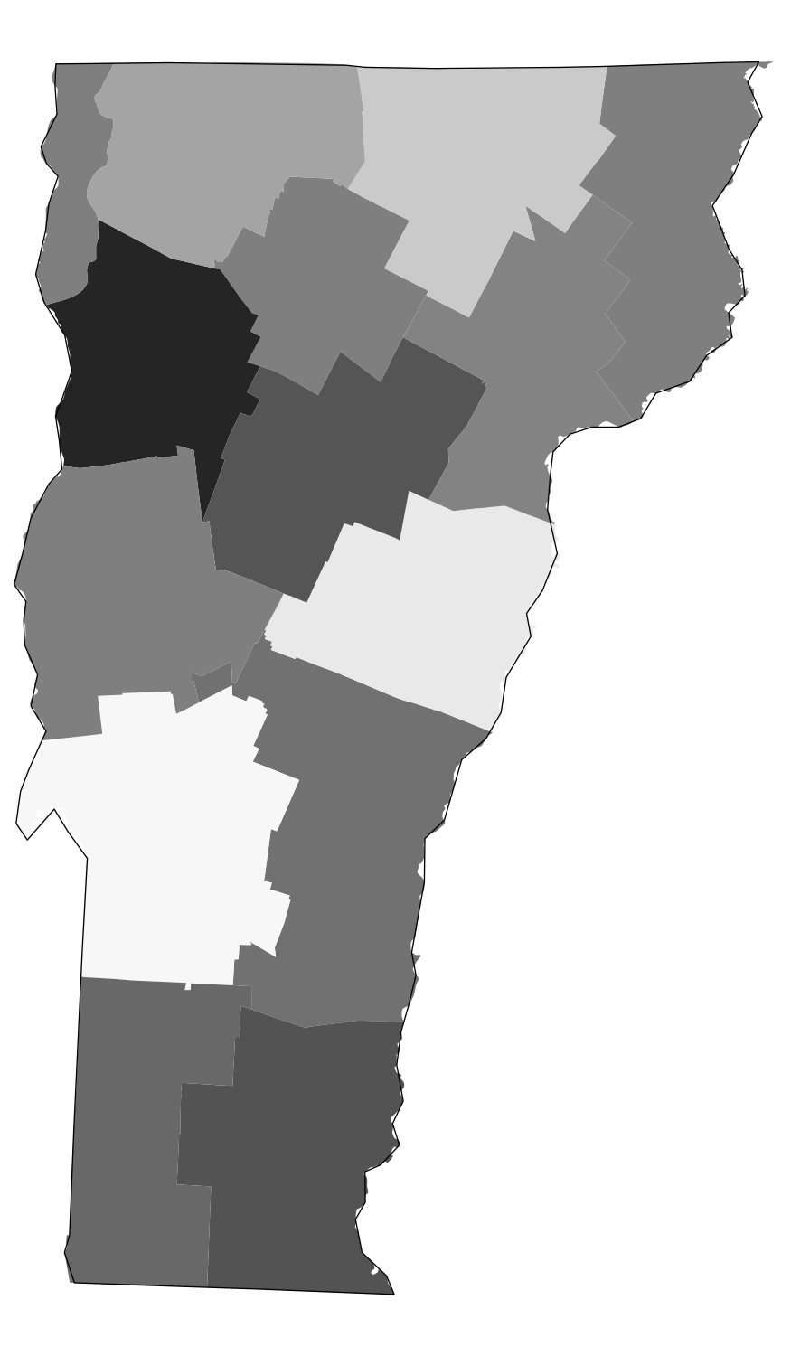
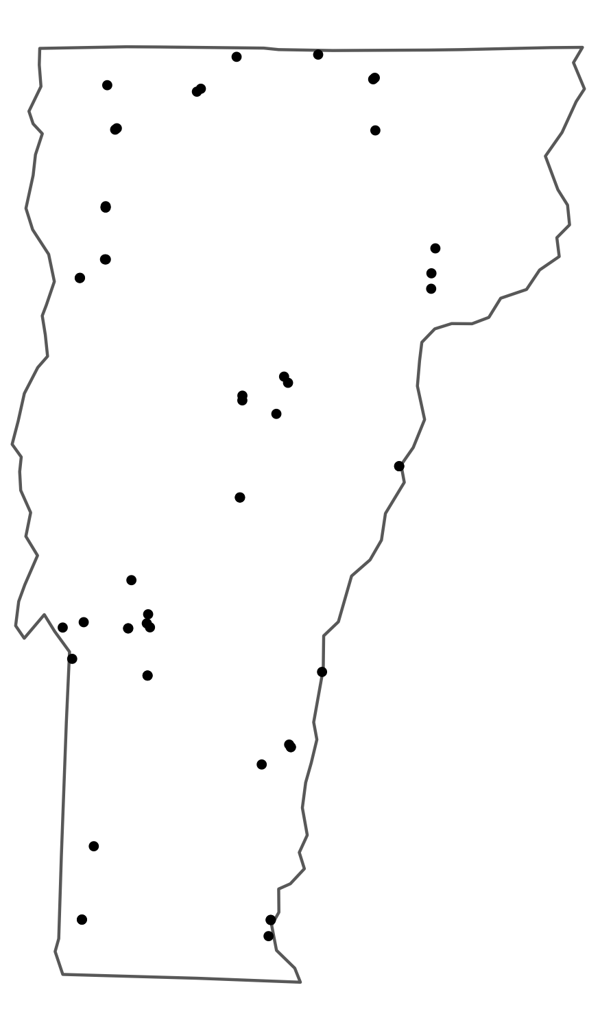
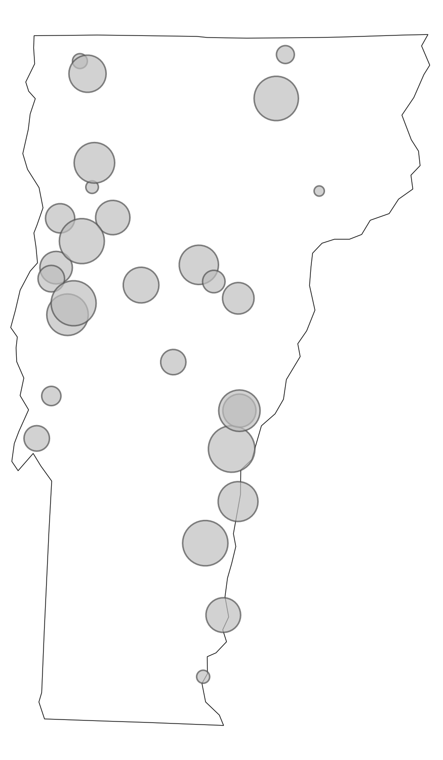
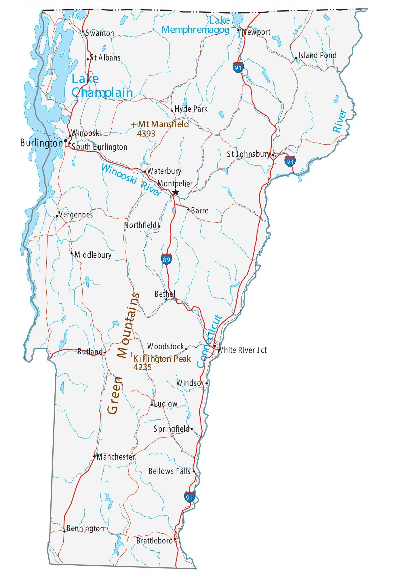
Choropleth: areas shaded by value

Dot map: one dot per unit

Proportional symbol: symbol size = quantity

Reference: orientation / context

Part 2: Mapping in ggplot2

Getting Boundary Data

• TIGER/Line files: the Census Bureau’s authoritative geographic boundary dataset, covering states, counties, tracts, roads, water features, and more
• tigris: an R package that downloads TIGER/Line files directly from the Census API and returns them as sf objects, ready to map

states_sf <- states(cb = TRUE, resolution = "20m") %>%
  filter(!STUSPS %in% c("AK", "HI", "PR", "VI", "GU", "AS", "MP"))

counties_sf <- counties(cb = TRUE, resolution = "20m") %>%
  filter(!STATEFP %in% c("02", "15", "72", "78", "66", "60", "69"))

• cb = TRUE: simplified cartographic boundary (better for maps)
• resolution = "20m": 1:20,000,000 scale (right for national maps)
• The filter removes Alaska, Hawaii, and territories

tigris has many other geographies too: tracts, block groups, places, county subdivisions (New England towns), school districts, congressional districts, ZIP codes, roads, water features. All come back as sf objects ready to use.

Your First Map

ggplot(states_sf) +
  geom_sf()

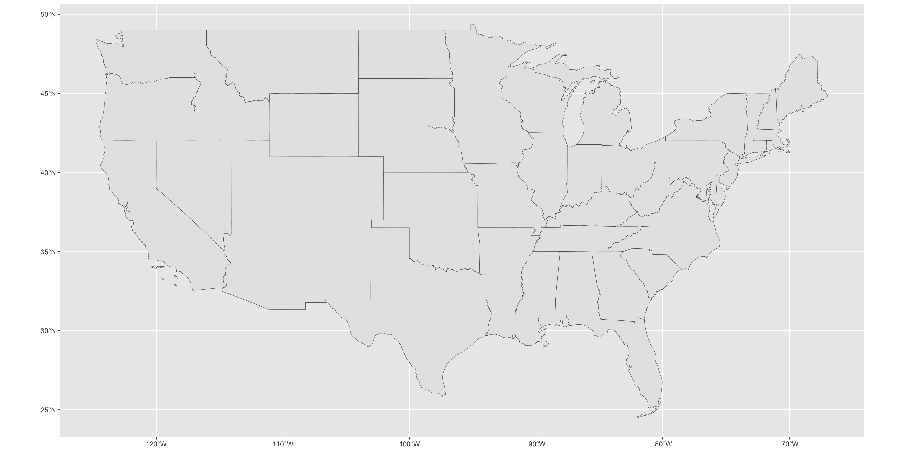
geom_sf() reads the geometry column and draws the shapes. But it looks flat and weird – let’s fix that.

Your First Map

Applying a Projection

ggplot(states_sf) +
  geom_sf() +
  coord_sf(crs = 5070)

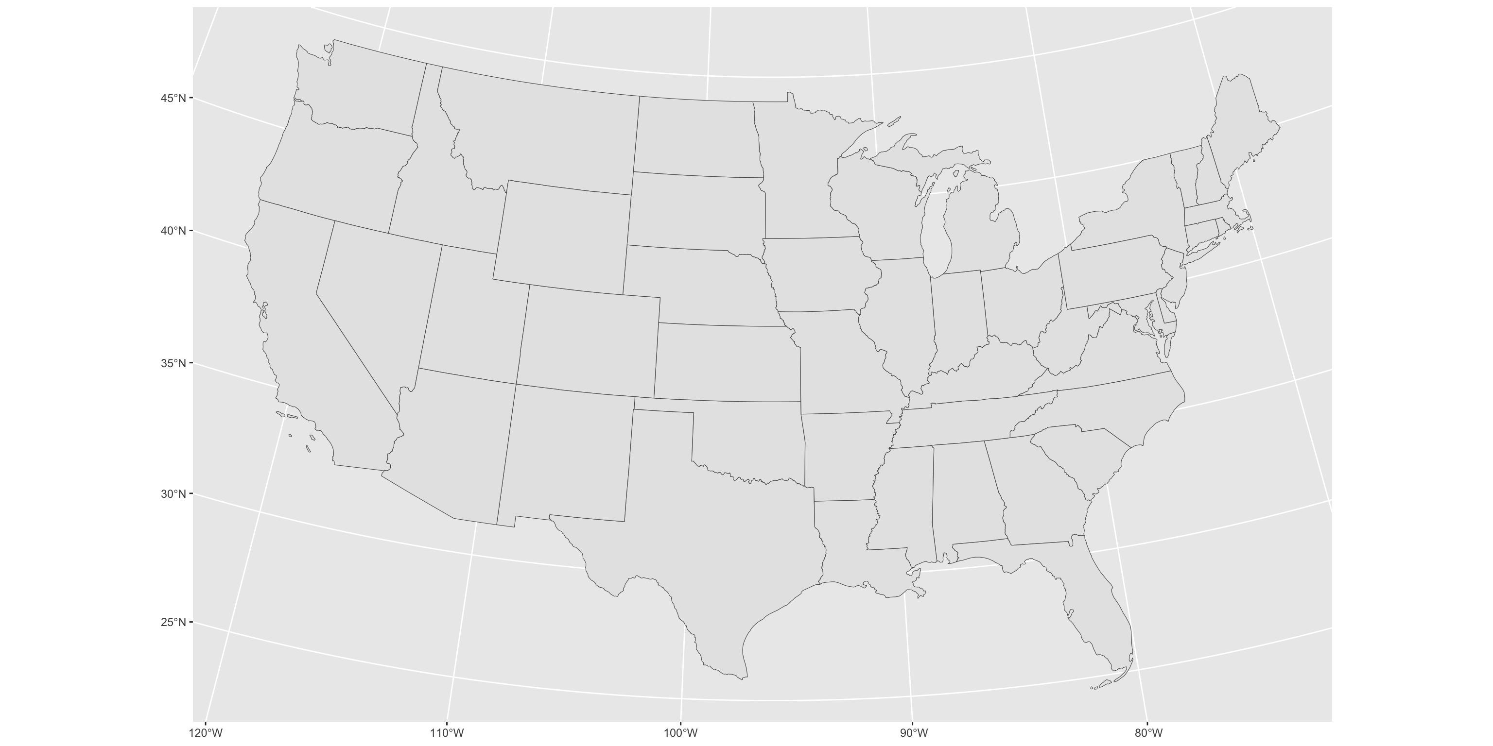
coord_sf() reprojects the visualization without modifying your data. This single line is the most impactful improvement you can make to a US national map.

Applying a Projection

Styling

ggplot(states_sf) +
  geom_sf(fill = "dodgerblue", color = "white", linewidth = 0.3) +
  coord_sf(crs = 5070) +
  theme_void()

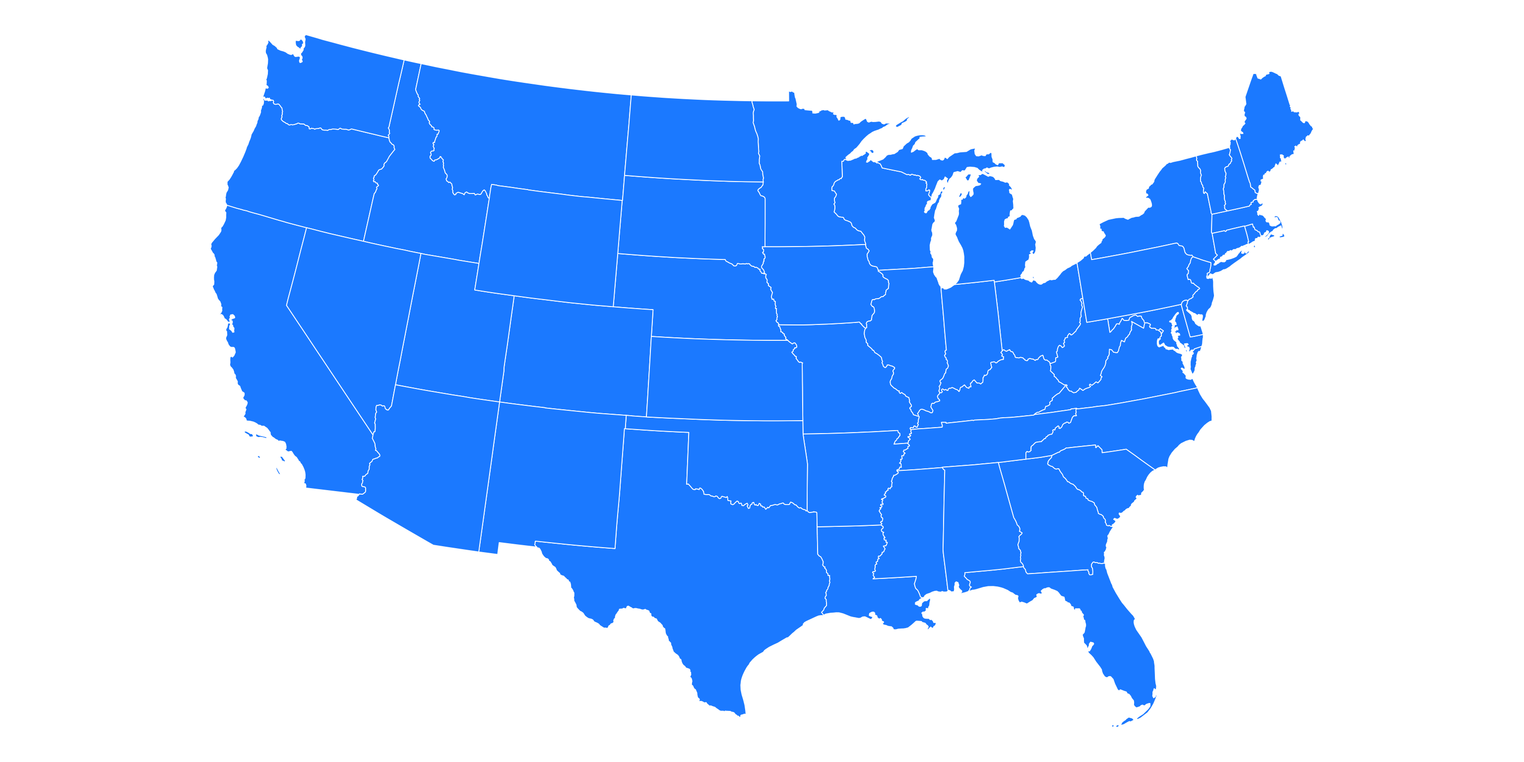
theme_void() removes axes, gridlines, and background – almost always the right choice for a finished map.

Styling

Zooming In: New England

An sf object filters like any data frame, so a regional map is one filter() away.

ne_states <- c("CT", "ME", "MA", "NH", "RI", "VT")

ne_sf          <- states_sf   %>% filter(STUSPS %in% ne_states)
ne_counties_sf <- counties_sf %>% filter(STUSPS %in% ne_states)

ne_crs <- 26986  # NAD83 / Massachusetts State Plane (Mainland), in meters

• ggplot() sets the map extent from the data, so the map zooms to New England on its own
• 5070 is centered on the middle of the country (96°W), so New England comes out tilted. A projection centered on the region (71.5°W) sits it upright

Real Data: LACE

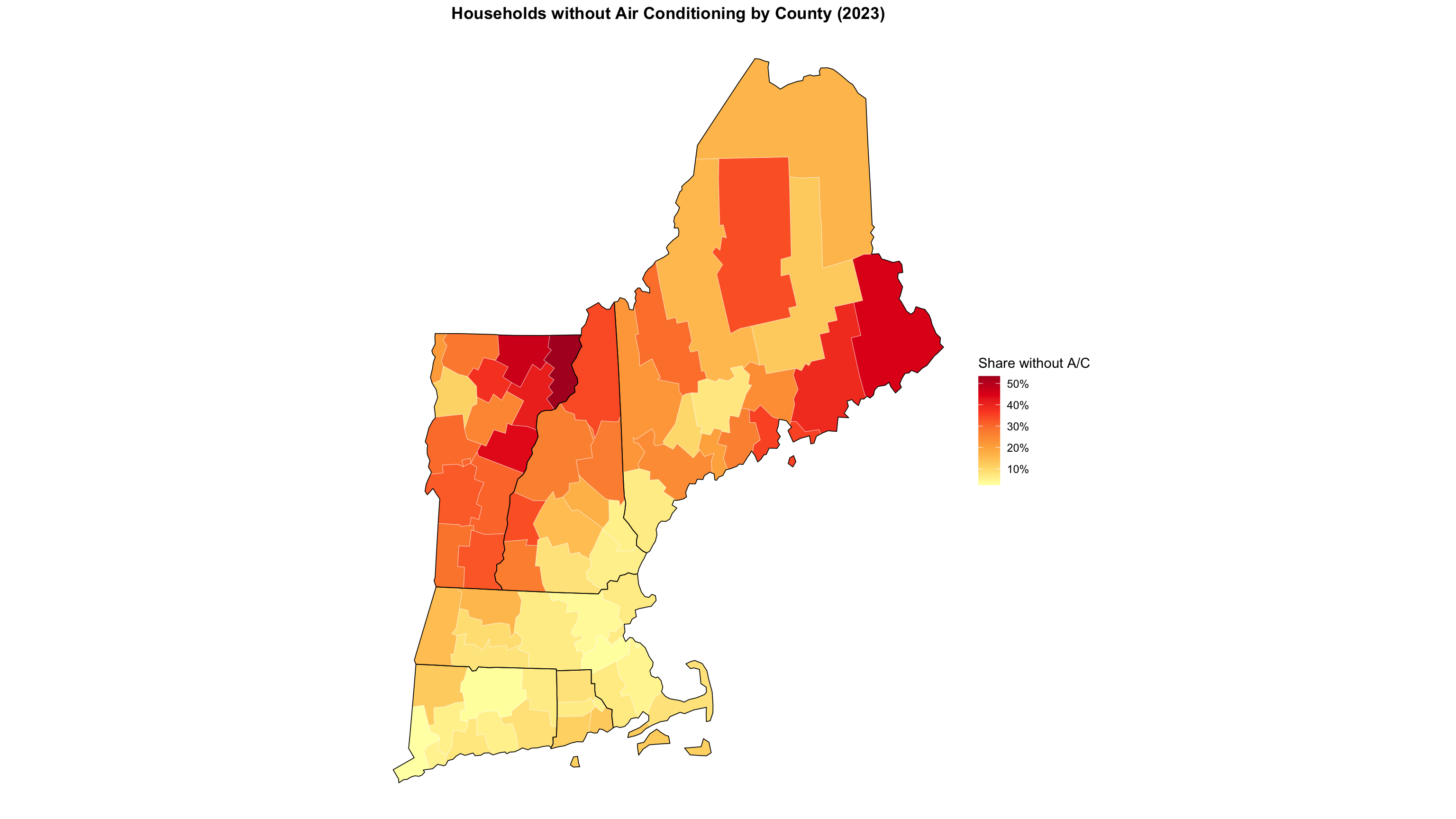
New from the Census Bureau: county-level estimates of households without air conditioning.

lace <- read_csv("https://www2.census.gov/programs-surveys/demo/datasets/lace/2023/LACE_23_County.csv") %>%
  mutate(GEOID = paste0(STATE, COUNTY))

lace_map <- ne_counties_sf %>%
  left_join(lace, by = "GEOID")

This is the standard workflow: get boundaries from tigris, join your data on GEOID, map it.

GEOID is the 5-character FIPS code: 2-digit state + 3-digit county, always zero-padded. This is the universal join key for any Census-derived county data. Northern New England has some of the lowest AC adoption in the country, which matters more every summer.

Building the Map Incrementally

ggplot(lace_map) +
  geom_sf(aes(fill = NO_AC_PE/100), color = "white", linewidth = 0.1) +
  geom_sf(data = ne_sf, fill = NA, color = "black", linewidth = 0.3) +
  coord_sf(crs = ne_crs) +
  scale_fill_distiller(
    palette = "YlOrRd", direction = 1,
    labels = percent, name = "Share without A/C"
  ) +
  theme_void() +
  theme(legend.position = "right",
        plot.title = element_text(face = "bold", hjust = .5)) +
  labs(title = "Households without Air Conditioning by County (2023)")

[Live demo.] In demo_script.R, start with most of these arguments commented out. Uncomment one at a time so the audience can see what each piece contributes to the finished map.

Building the Map Incrementally

Color Scale Options

# Sequential (one hue, light to dark)
scale_fill_distiller(palette = "YlOrRd", direction = 1)
scale_fill_viridis_c(option = "rocket")

# Diverging (two hues, use when 0 means something)
scale_fill_distiller(palette = "RdBu", direction = 1)

# Right-skewed data: log-transform the scale
scale_fill_viridis_c(trans = "log10", labels = scales::comma)

Avoid rainbow palettes (rainbow(), jet). They are not perceptually uniform and create false visual boundaries in your data.

• ColorBrewer (colorbrewer2.org) — designed by cartographer Cynthia Brewer, it provides rigorously tested sequential, diverging, and qualitative palettes optimized for maps. No need to reinvent the wheel; the cartographers already laid the groundwork.

Part 3: Census Data

tidycensus

tidycensus pulls Census Bureau data directly into R, with geometry attached if you want it.

# one-time setup -- free key at api.census.gov/data/key_signup.html
census_api_key("YOUR_KEY_HERE", install = TRUE)

Covers: Decennial Census, ACS 1-year and 5-year, and more

ACS data is estimated, not a headcount. The smaller the geography, the larger the margin of error. A tract-level estimate has a much wider confidence interval than a county-level one, and small New England towns are noisier still.

Finding Variables

v24 <- load_variables(2024, "acs5", cache = TRUE)

v24 %>%
  filter(str_detect(concept, regex("heating fuel", ignore_case = TRUE))) %>%
  select(name, label, concept)

# A tibble: 34 × 3
   name       label                                                      concept
   <chr>      <chr>                                                      <chr>  
 1 B25040_001 Estimate!!Total:                                           House …
 2 B25040_002 Estimate!!Total:!!Utility gas                              House …
 3 B25040_003 Estimate!!Total:!!Bottled or tank gas (propane, butane, e… House …
 4 B25040_004 Estimate!!Total:!!Electricity                              House …
 5 B25040_005 Estimate!!Total:!!Fuel oil, kerosene, etc.                 House …
 6 B25040_006 Estimate!!Total:!!Coal or coke                             House …
 7 B25040_007 Estimate!!Total:!!Wood                                     House …
 8 B25040_008 Estimate!!Total:!!Solar energy                             House …
 9 B25040_009 Estimate!!Total:!!Other fuel                               House …
10 B25040_010 Estimate!!Total:!!No fuel used                             House …
# ℹ 24 more rows

There are ~28,000 ACS 5-year variables. load_variables() + str_detect() is how you find what you need.

Pulling Heating Fuel Data with Geometry

heating_oil <- get_acs(
  geography = "county",
  state     = ne_states,
  variables = c(oil   = "B25040_005",
                total = "B25040_001"),
  year      = 2024,
  geometry  = TRUE
) %>%
  select(GEOID, NAME, variable, estimate) %>%
  pivot_wider(names_from = variable, values_from = estimate) %>%
  mutate(oil_pct = oil / total)

geometry = TRUE is the killer feature: one call returns data and boundaries together.

B25040_005 is “Fuel oil, kerosene, etc.” New England is the one region of the country where heating oil is still a mainstream fuel, which ties household budgets directly to global distillate prices every winter.

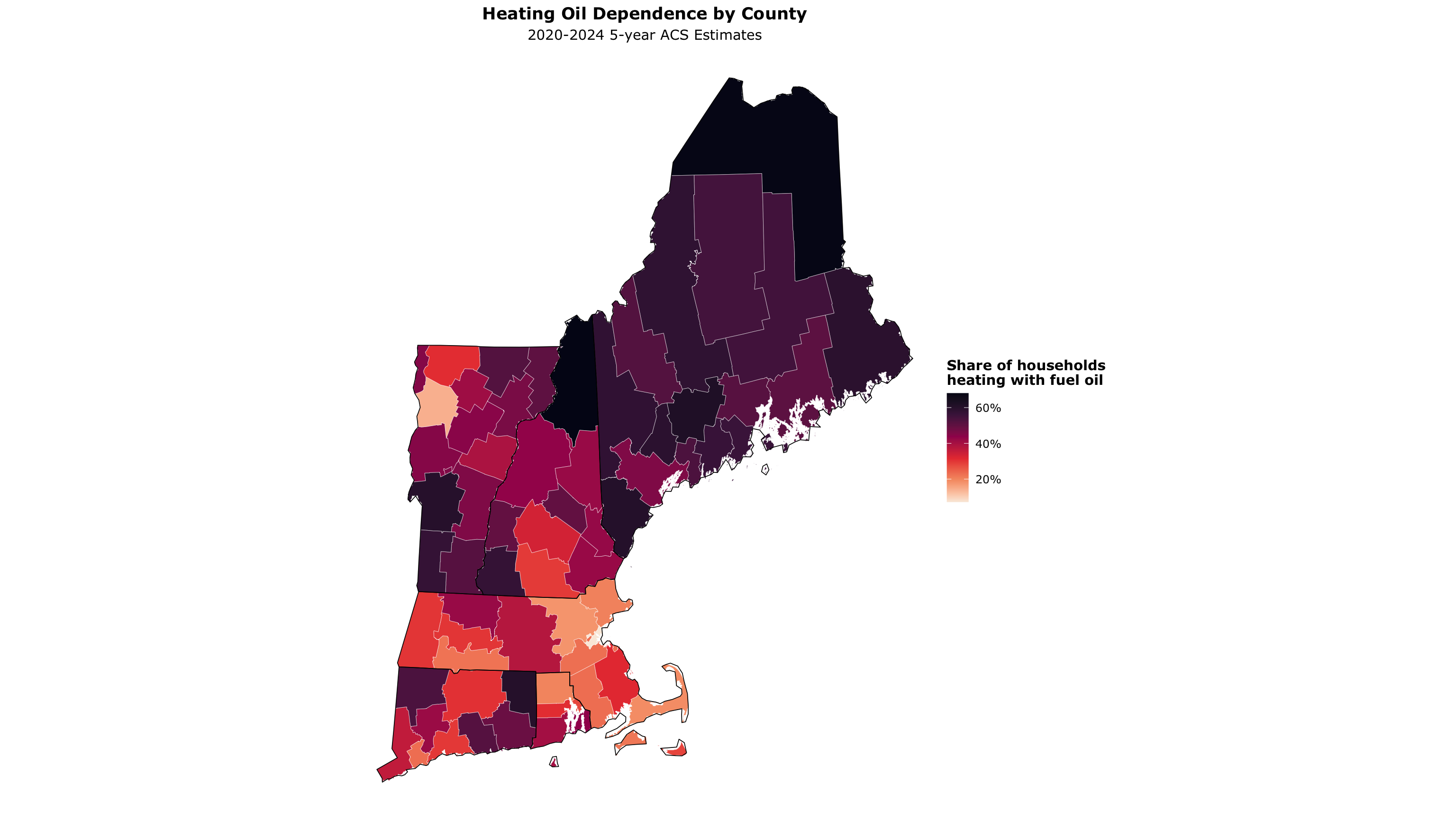
Heating Oil Dependence by County

ggplot(heating_oil) +
  geom_sf(aes(fill = oil_pct), color = "white", linewidth = 0.1) +
  geom_sf(data = ne_sf, fill = NA, color = "black", linewidth = 0.3) +
  coord_sf(crs = ne_crs) +
  scale_fill_viridis_c(
    name = "Share of households\nheating with fuel oil",
    labels = percent_format(accuracy = 1),
    option = "rocket",
    direction = -1
  ) +
  theme_void(base_family = "Verdana") +
  theme(legend.title = element_text(face = "bold"),
        plot.title = element_text(face = "bold", hjust = .5),
        plot.subtitle = element_text(hjust = .5)) +
  labs(title = "Heating Oil Dependence by County",
       subtitle = "2020-2024 5-year ACS Estimates")

Heating Oil Dependence by County

Going Smaller: Census Tracts

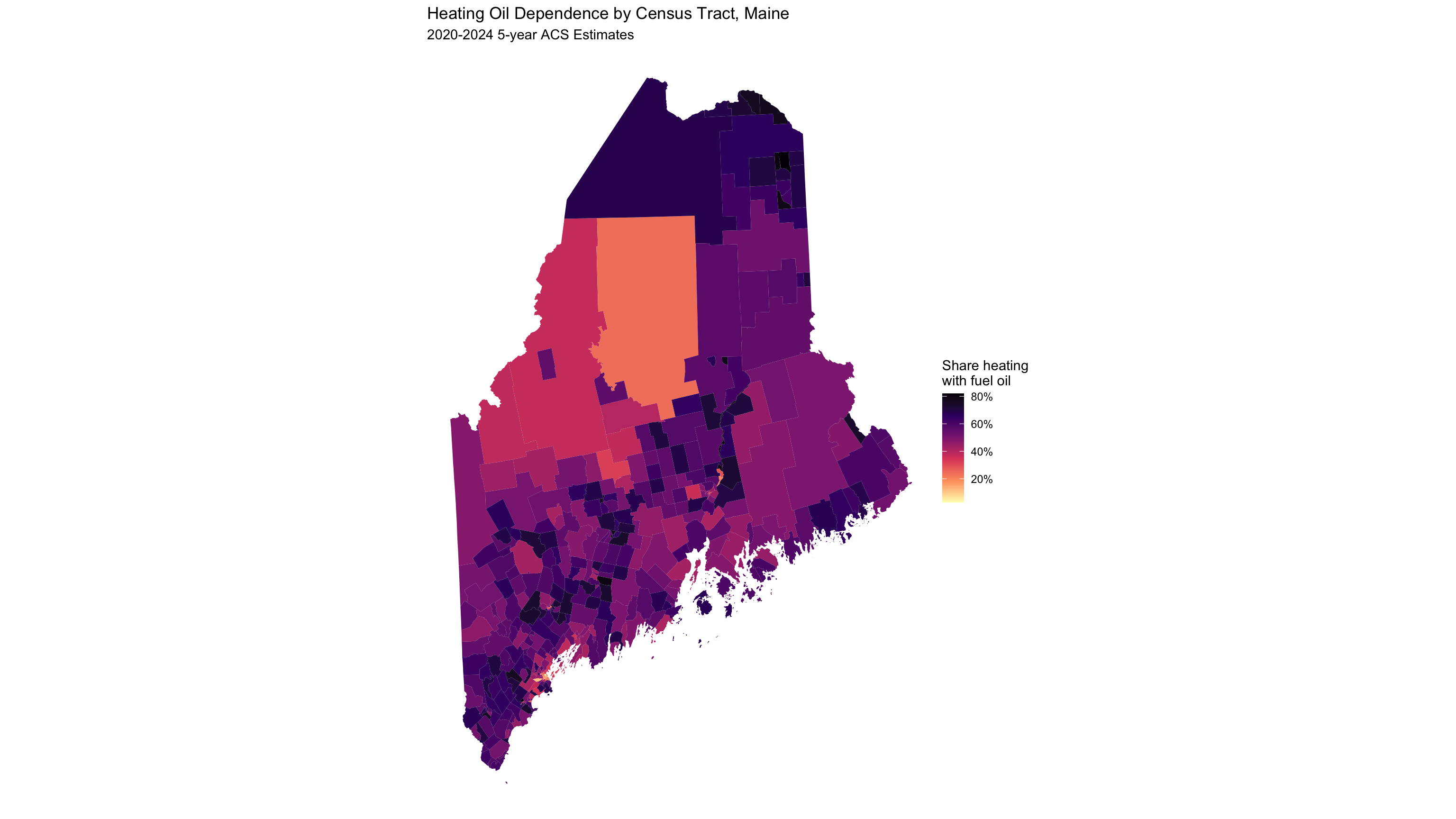
Change geography = "county" to geography = "tract":

get_acs(
  geography = "tract", state = "ME",
  variables = c(oil = "B25040_005", total = "B25040_001"),
  year = 2024, geometry = TRUE
) %>%
  select(GEOID, NAME, variable, estimate) %>%
  pivot_wider(names_from = variable, values_from = estimate) %>%
  mutate(oil_pct = oil / total) %>%
  ggplot() +
  geom_sf(aes(fill = oil_pct), color = NA) +
  coord_sf(crs = ne_crs) +
  scale_fill_viridis_c(option = "A", direction = -1,
                       name = "Share heating\nwith fuel oil",
                       labels = percent_format(accuracy = 1),
                       na.value = "grey90") +
  theme_void() +
  labs(title = "Heating Oil Dependence by Census Tract, Maine",
       subtitle = "2020-2024 5-year ACS Estimates")

Everything is the same except geography and state. tidycensus supports county, tract, block group, place, county subdivision, ZCTA, and more. Portland and Bangor stand out as the places where natural gas service reaches.

Going Smaller: Census Tracts

A New England Quirk: Connecticut

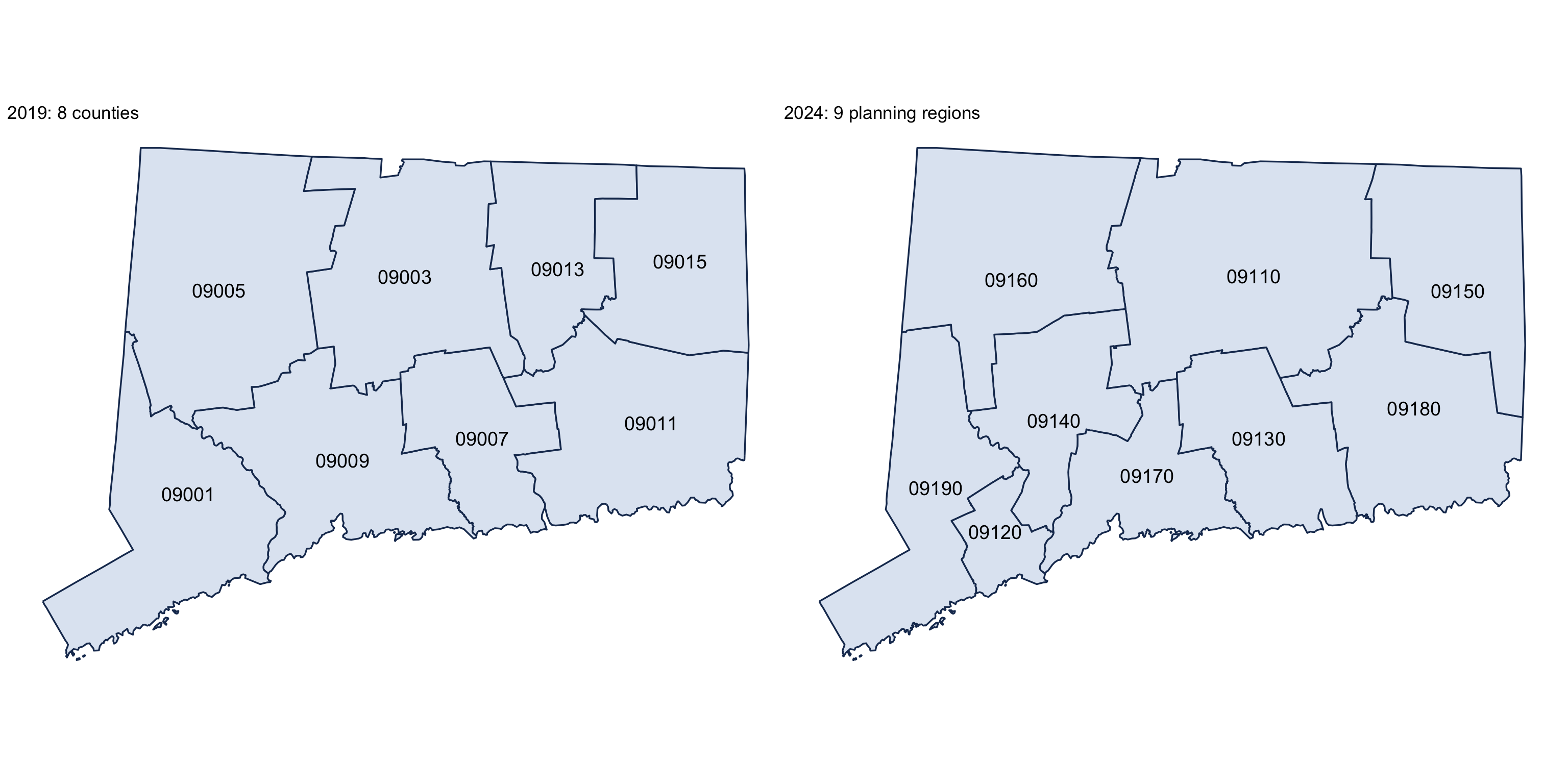
In 2022 the Census Bureau replaced Connecticut’s 8 counties with 9 planning regions.

ct_2019 <- counties(state = "CT", cb = TRUE, year = 2019)
ct_2024 <- counties(state = "CT", cb = TRUE, year = 2024)

ct_map <- function(x, title) {
  ggplot(x) +
    geom_sf(fill = "#dfe7f2", color = "#1b365d", linewidth = 0.6) +
    geom_sf_text(aes(label = GEOID), size = 5) +
    coord_sf(crs = ne_crs) +
    theme_void() +
    labs(title = title)
}

ct_map(ct_2019, "2019: 8 counties") + ct_map(ct_2024, "2024: 9 planning regions")

The boundaries and the GEOIDs changed (09001 → 09110–09190), so any county panel that spans 2022 breaks in Connecticut.

Most economists find this out when a merge silently drops Connecticut. The Census Bureau publishes a crosswalk, but for a lot of work the better answer is to use towns, which did not change. That’s next.

A New England Quirk: Connecticut

Towns: County Subdivisions

In New England, towns are the unit that matters. Census calls them county subdivisions.

wfh_towns <- function(year, geometry = FALSE) {
  map_dfr(ne_states, \(st) get_acs(
    geography = "county subdivision", state = st, year = year,
    variables = c(wfh = "B08301_021", workers = "B08301_001"),
    geometry = geometry
  )) %>%
    select(GEOID, NAME, variable, estimate) %>%
    pivot_wider(names_from = variable, values_from = estimate) %>%
    filter(workers > 0) %>%
    mutate(wfh_pct = wfh / workers)
}

wfh_2019 <- wfh_towns(2019)
wfh_2024 <- wfh_towns(2024, geometry = TRUE)

get_acs() only fetches county subdivision geometry one state at a time, so we loop with map_dfr().

Joining Across the Connecticut Break

sum(!wfh_2024$GEOID %in% wfh_2019$GEOID)

[1] 182

A town GEOID embeds its county, so every Connecticut town “moved.” The fix is to join on state FIPS + the 5-digit town code, which never changed:

town_key <- function(geoid) paste0(str_sub(geoid, 1, 2), str_sub(geoid, 6, 10))

wfh_towns_sf <- wfh_2024 %>%
  mutate(key = town_key(GEOID)) %>%
  left_join(wfh_2019 %>% transmute(key = town_key(GEOID), wfh_pct_2019 = wfh_pct),
            by = "key") %>%
  rename(wfh_pct_2024 = wfh_pct)

Finding Better Breaks: Jenks

Skewed data looks like one color with a linear scale. Jenks natural breaks fix that.

combined <- c(wfh_towns_sf$wfh_pct_2019, wfh_towns_sf$wfh_pct_2024)

brks <- classIntervals(combined[!is.na(combined)], n = 5, style = "jenks")$brks %>%
  round(2)

pal <- brewer.pal(length(brks), "YlGnBu")

Using the combined distribution ensures both maps share the same color scale.

Keeping Web Maps Light

Interactive maps ship every vertex to the browser. Simplify what the widget embeds:

wfh_web <- wfh_towns_sf %>%
  st_transform(4326) %>%
  ms_simplify(keep = 0.35, keep_shapes = TRUE)

• keep = 0.35 keeps 35% of the vertices; shared borders stay shared, so towns still tile
• Keep full resolution for analysis and static maps

Comparing Maps with compare()

wfh_map <- function(column, title) {
  maplibre(bounds = ne_sf, style = carto_style("voyager")) %>%
    add_source(id = "towns", data = wfh_web) %>%
    add_fill_layer(id = column, source = "towns",
      fill_color = interpolate(column = column,
                               values = brks, stops = pal, na_color = "lightgrey"),
      fill_opacity = 0.85, tooltip = "NAME") %>%
    add_line_layer(id = "states", source = ne_sf, line_width = .5) %>%
    add_continuous_legend(title, values = percent(brks), colors = pal,
                          position = "top-left")
}

compare(wfh_map("wfh_pct_2019", "Work from home, 2015-2019"),
        wfh_map("wfh_pct_2024", "Work from home, 2020-2024"),
        height = "900px")

Drag the slider. Remote work roughly doubled nearly everywhere, but look at the ring around Boston and the Upper Valley versus the old mill towns. Tiny towns swing wildly because the ACS margins of error are huge there; zoom in and hover to show one.

Comparing Maps with compare()

Part 4: Point Data and GIS

From Table to Map

Any table with latitude and longitude columns can become a spatial dataset.

schools <- read_csv("https://andrewvanleuven.github.io/bostonfed_neppc/data/public_schools.csv")
glimpse(schools)

Rows: 4,603
Columns: 8
$ ncessch   <chr> "090000201136", "090000201137", "090000201138", "09000020113…
$ name      <chr> "A. I. Prince Technical High School", "Bullard-Havens Techni…
$ city      <chr> "Hartford", "Bridgeport", "New Britain", "Groton", "Hamden",…
$ state     <chr> "CT", "CT", "CT", "CT", "CT", "CT", "CT", "CT", "CT", "CT", …
$ county    <chr> "Capitol Planning Region", "Greater Bridgeport Planning Regi…
$ locale    <chr> "City", "City", "Suburb", "Rural", "Suburb", "Suburb", "Subu…
$ latitude  <dbl> 41.74248, 41.19971, 41.68677, 41.34212, 41.34246, 41.33504, …
$ longitude <dbl> -72.70677, -73.16397, -72.80608, -72.01666, -72.94175, -73.0…

Source: NCES EDGE public school geocodes, 2024-25 school year. The locale field is NCES’s urban-centric classification: city, suburb, town, rural.

st_as_sf(): Adding Geometry

schools_sf <- schools %>%
  st_as_sf(coords = c("longitude", "latitude"), crs = 4326, remove = FALSE) %>%
  st_transform(crs = ne_crs) %>%
  mutate(locale = factor(locale, levels = c("City", "Suburb", "Town", "Rural")))

st_as_sf() turns lat/lon columns into a geometry column. After that, it’s a normal sf object.

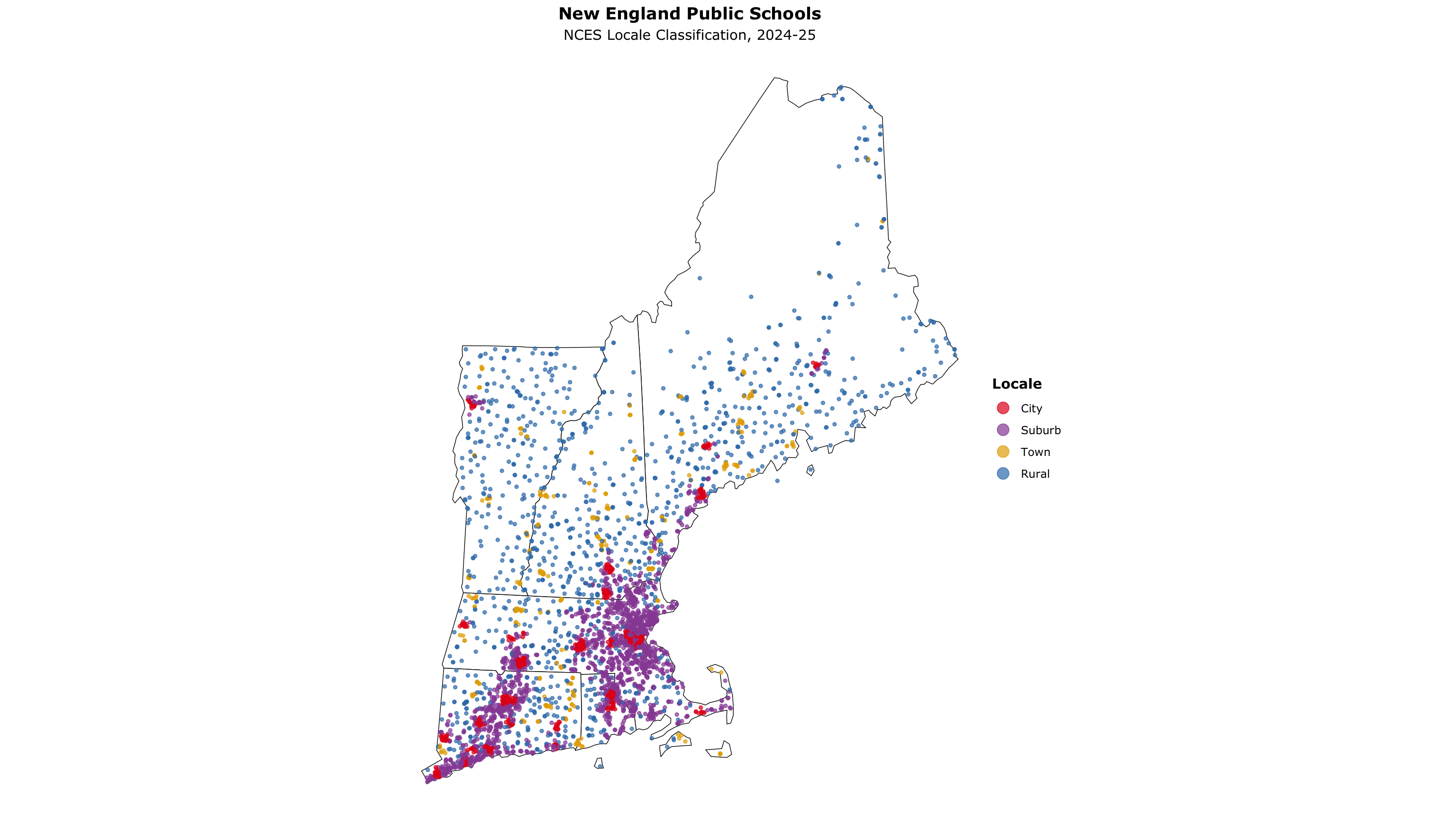
Public Schools by Locale

ggplot() +
  geom_sf(data = ne_sf, fill = "white", color = "black", linewidth = .25) +
  geom_sf(data = schools_sf, aes(color = locale), size = 1, alpha = .7) +
  scale_color_manual(values = c("#e41a1c", "#984ea3", "#e6ab02", "#377eb8"), name = "Locale") +
  coord_sf(crs = ne_crs) +
  theme_void(base_family = "Verdana") +
  theme(legend.title = element_text(face = "bold"),
        plot.subtitle = element_text(hjust = .5),
        plot.title = element_text(face = "bold", hjust = .5)) +
  guides(color = guide_legend(override.aes = list(size = 4))) +
  labs(title = "New England Public Schools",
       subtitle = "NCES Locale Classification, 2024-25")

Public Schools by Locale

Categorical Point Maps with mapgl

grocery_stores <- read_csv("https://andrewvanleuven.github.io/bostonfed_neppc/data/grocery_stores.csv") %>%
  st_as_sf(wkt = "geometry_wkt", crs = 4326) %>%
  mutate(tooltip = glue("<b>{name}</b><br>{city_name}, {state}"))

grocers <- c("Market Basket", "Hannaford", "Stop & Shop", "Shaw's", "Price Chopper")
grocer_colors <- c("#c8102e", "#5a8f29", "#6c2c91", "#0072ce", "#f39200")

maplibre(style = carto_style("positron"), bounds = ne_sf) %>%
  add_circle_layer(
    id = "poi-grocery", source = grocery_stores,
    circle_color = match_expr("name", values = grocers, stops = grocer_colors),
    circle_radius = 5, circle_stroke_color = "#ffffff",
    circle_stroke_width = .6, circle_opacity = 0.85, tooltip = "tooltip"
  ) %>%
  add_line_layer(id = "states", source = ne_sf, line_width = .5) %>%
  add_categorical_legend(
    legend_title = "New England Supermarket Chains",
    values = grocers, colors = grocer_colors,
    patch_shape = "circle", position = "bottom-right",
    layer_id = "poi-grocery", interactive = TRUE
  )

Source: Overture Maps Foundation. Click the legend entries to toggle chains. The territories barely overlap: Stop & Shop in southern New England, Hannaford in Maine, Price Chopper along the New York border, Market Basket radiating out of the Merrimack Valley.

Categorical Point Maps with mapgl

Dunkin’ vs. Starbucks

coffee_shops <- read_csv("https://andrewvanleuven.github.io/bostonfed_neppc/data/coffee_shops.csv") %>%
  st_as_sf(wkt = "geometry_wkt", crs = 4326) %>%
  mutate(tooltip = glue("<b>{name}</b><br>{city_name}, {state}"))

maplibre(style = carto_style("positron"), bounds = ne_sf) %>%
  add_circle_layer(
    id           = "poi-coffee",
    source       = coffee_shops,
    circle_color = match_expr(
      "name",
      values = c("Dunkin'", "Starbucks"),
      stops  = c("#FF671F", "#00704A")
    ),
    circle_radius       = 4,
    circle_stroke_color = "white",
    circle_stroke_width = .4,
    circle_opacity      = 0.8,
    tooltip             = "tooltip"
  ) %>%
  add_categorical_legend(
    legend_title = "Coffee Chains",
    values       = c("Dunkin'", "Starbucks"),
    colors       = c("#FF671F", "#00704A"),
    patch_shape  = "circle",
    position     = "bottom-right",
    layer_id     = "poi-coffee",
    interactive  = TRUE
  )

Source: Overture Maps Foundation. Roughly 2,700 Dunkin’ locations to 750 Starbucks across the region. Toggle Dunkin’ off to see how Starbucks hugs the interstates and the wealthier Boston suburbs.

Dunkin’ vs. Starbucks

st_intersection: Points in Polygons

town_pop_2020 <- map_dfr(ne_states, \(st) get_decennial(
  geography = "county subdivision", state = st,
  variables = "P1_001N", year = 2020, geometry = TRUE
)) %>%
  filter(value > 0) %>%
  st_transform(ne_crs) %>%
  select(town_id = GEOID, town = NAME, pop20 = value)

dunkin_by_town <- coffee_shops %>%
  filter(name == "Dunkin'") %>%
  st_transform(ne_crs) %>%
  st_intersection(town_pop_2020) %>%
  st_drop_geometry() %>%
  count(town_id, name = "dunkins")

dunkin_sf <- town_pop_2020 %>%
  left_join(dunkin_by_town, by = "town_id") %>%
  replace_na(list(dunkins = 0)) %>%
  mutate(dunkins_per_10k = dunkins / pop20 * 10000)

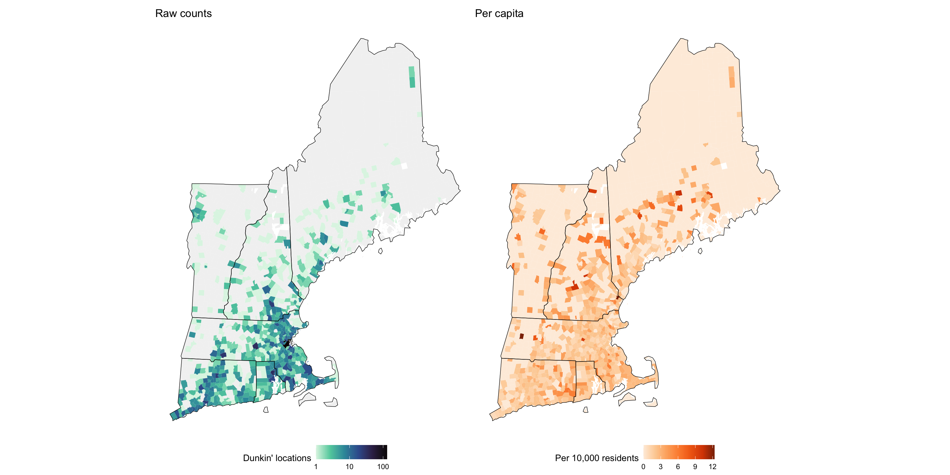
Raw Counts vs Per Capita

p1 <- ggplot() +
  geom_sf(data = dunkin_sf, aes(fill = dunkins), color = NA) +
  geom_sf(data = ne_sf, color = "black", linewidth = .25, fill = NA) +
  coord_sf(crs = ne_crs) +
  scale_fill_viridis_c(option = "mako", name = "Dunkin' locations",
                       trans = "log10", direction = -1, na.value = "gray95") +
  theme_void() + theme(legend.position = "bottom") +
  labs(title = "Raw counts")

p2 <- ggplot() +
  geom_sf(data = dunkin_sf, aes(fill = dunkins_per_10k), color = NA) +
  geom_sf(data = ne_sf, color = "black", linewidth = .25, fill = NA) +
  coord_sf(crs = ne_crs) +
  scale_fill_distiller(palette = "Oranges", name = "Per 10,000 residents",
                       direction = 1, na.value = "white") +
  theme_void() + theme(legend.position = "bottom") +
  labs(title = "Per capita")

p1 + p2

Raw counts favor dense, populous places: Boston has 131 Dunkin’s. Per capita, the leaders are small towns on highway exits, like Tilton NH on I-93, where travelers inflate the numerator. Always normalize for a choropleth unless you’re specifically making a point about total volume, and think about whose population the denominator really is.

Raw Counts vs Per Capita

Buffer Analysis: st_buffer

maine_grocery_buffers <- grocery_stores %>%
  filter(state == "ME") %>%
  st_transform(26919) %>%
  st_buffer(10 * 1609.34) %>%
  st_transform(4326)

maplibre(bounds = filter(ne_sf, STUSPS == "ME"),
         style = carto_style("positron")) %>%
  add_fill_layer(
    id = "buffers", source = maine_grocery_buffers,
    fill_color = "#202020", fill_opacity = 0.4
  )

st_buffer() creates a polygon a fixed distance around each point. CRS 26919 (UTM zone 19N) uses meters, so 10 miles = 16,093 meters.

Everything outside the gray is more than 10 miles from a major supermarket chain. That’s about two-thirds of Maine by area, though far less of it by population. Independent grocers fill some of the gap, and they aren’t in this chain-only dataset.

Buffer Analysis: st_buffer

From Dense Points to Heatmap

ma_dunkin <- coffee_shops %>%
  filter(state == "MA", name == "Dunkin'") %>%
  st_jitter(factor = 0.0001)

maplibre(style = carto_style("positron"),
         bounds = filter(ne_sf, STUSPS == "MA")) %>%
  add_circle_layer(
    id = "poi-dunkin", source = ma_dunkin,
    circle_color = "#FF671F", circle_stroke_color = "white", circle_stroke_width = 1
  ) %>%
  add_heatmap_layer(
    id = "heatmap", source = ma_dunkin, heatmap_radius = 25,
    heatmap_color = interpolate(
      property = "heatmap-density", values = seq(0, 1, 0.2),
      stops = c("transparent", magma(5))
    )
  )

From Dense Points to Heatmap

More Things sf Can Do

st_distance()        # distance between features (in CRS units)
st_nearest_feature() # index of the nearest feature in another layer
st_centroid()        # geometric center of a polygon
st_area()            # area of a polygon (in CRS units)
st_union()           # merge / dissolve geometries into one
st_bbox()            # bounding box of a layer
st_crop()            # clip features to a rectangular extent
st_within()          # is feature A fully inside feature B?
st_touches()         # do features share a boundary?

sf cheat sheet: rstudio.github.io/cheatsheets/sf.pdf

More Examples of Spatial Data Visualization in R

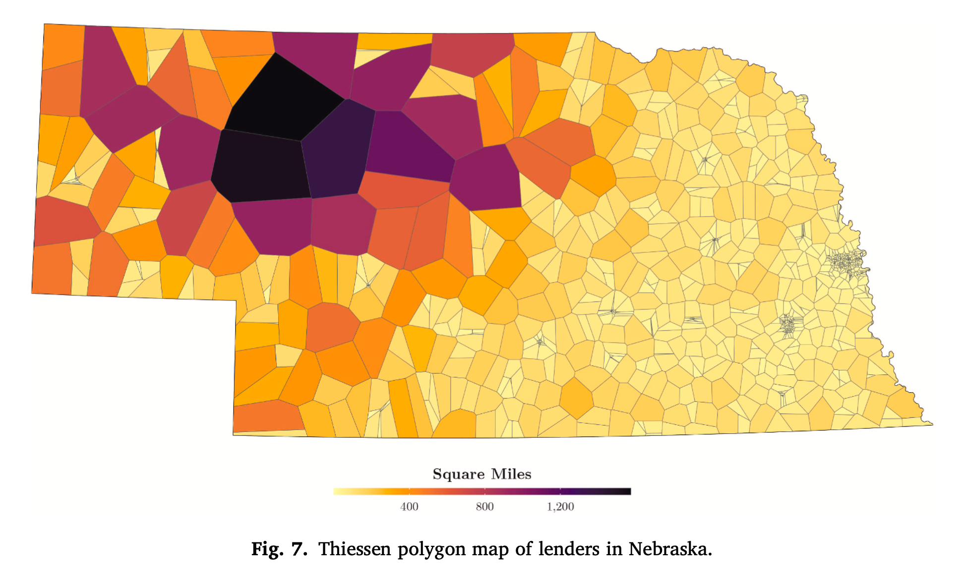
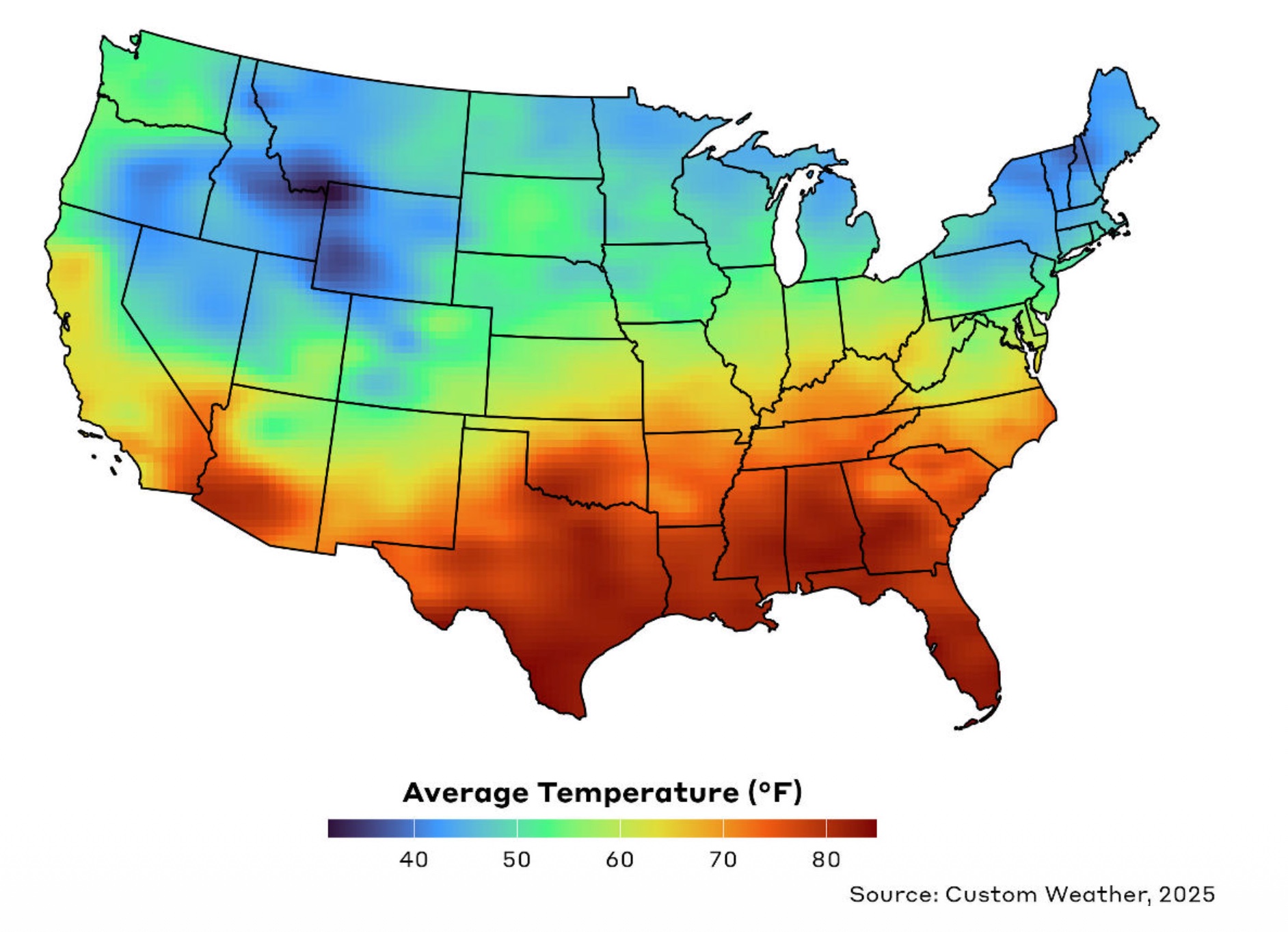
More Examples of Spatial Data Visualization in R

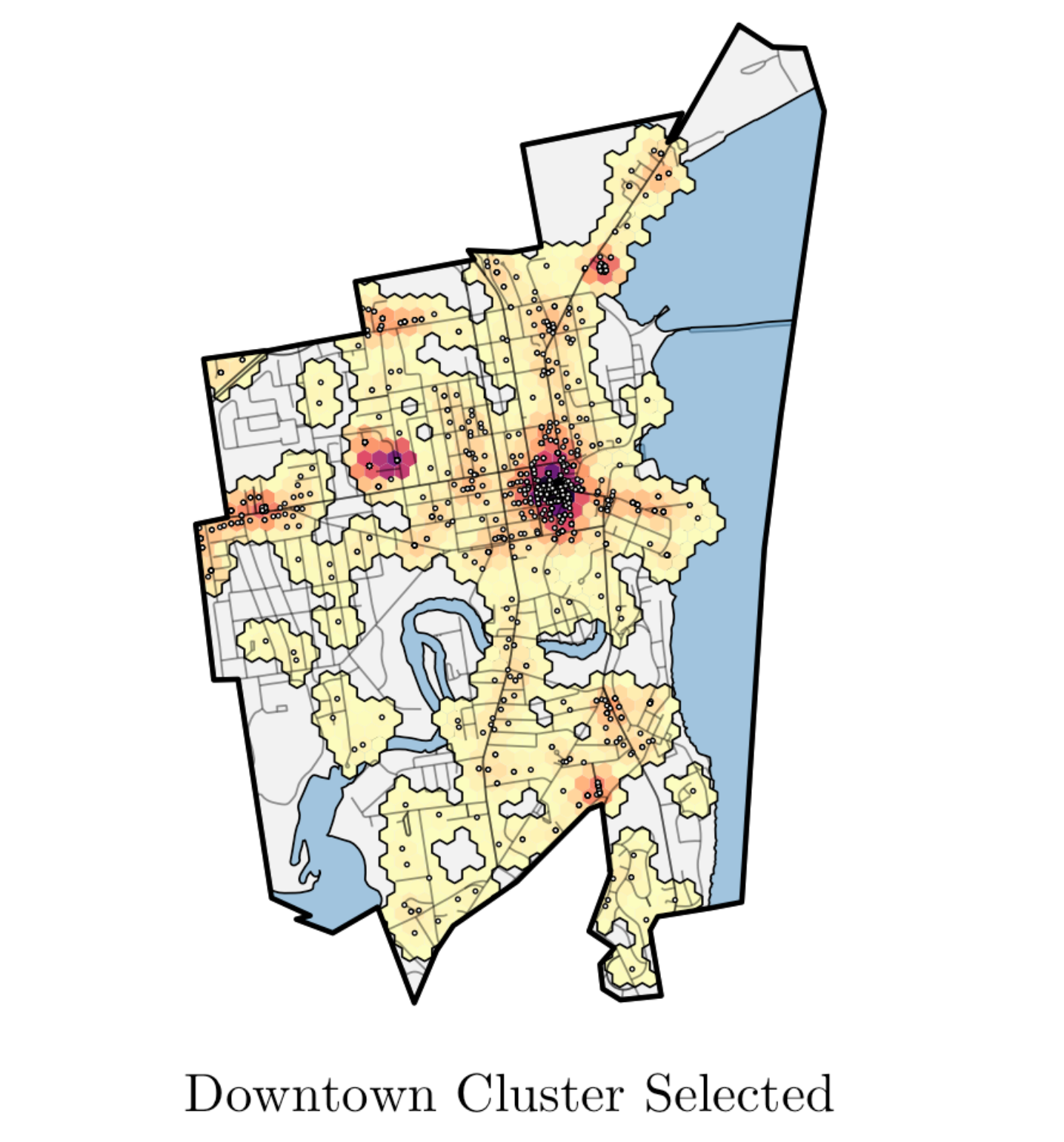
More Examples of Spatial Data Visualization in R

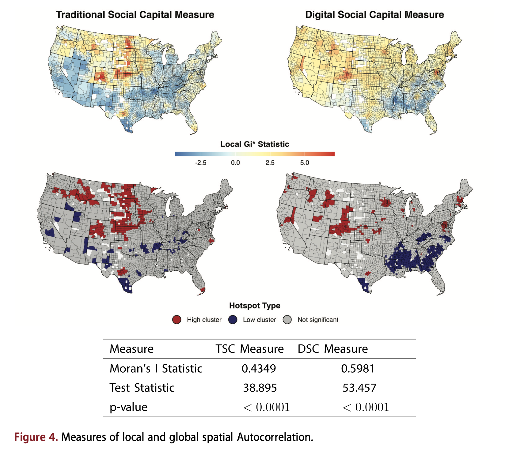
More Examples of Spatial Data Visualization in R

Wrap Up

What We Covered

1. Mapping basics: vector vs. raster data, coordinate reference systems, map types
2. ggplot2 maps: tigris for boundaries, geom_sf(), projections, color scales, choropleth maps
3. Census data: tidycensus with geometry, counties to tracts to towns, Connecticut’s planning regions, classification breaks, side-by-side map comparison
4. Point data and GIS operations: st_as_sf(), categorical styling, spatial joins, counts vs. rates, buffer analysis, heatmaps

Thank You

Andrew Van Leuven University of Vermont

andrew.vanleuven@uvm.edu

https://andrewvanleuven.com

Questions?

Thank Jeff and the NEPPC team.