Introduction to Maps

USDA AMS/AAEA GSS Local Food Economics Data Visualization Challenge

Andrew Van Leuven | University of Vermont

June 4, 2026

Follow Along

Scan to download the R script used in today’s demo:

GitHub Link: https://github.com/andrewvanleuven/andrewvanleuven.github.io/blob/main/aaea_webinar/demo_script.R

Agenda

1. Mapping basics
2. Mapping in ggplot2
3. Data from Census and NASS QuickStats
4. Point data and basic GIS operations

Welcome everyone. We have about 60 minutes together. We’ll do live demos along the way using demo_script.R – feel free to open it and follow along in RStudio. Questions at the end.

Packages We’ll Use Today

install.packages(c(
  "tidyverse",   # data manipulation + ggplot2
  "sf",          # spatial data in R
  "tigris",      # US Census boundary files
  "tidycensus",  # Census + ACS data with geometry
  "rnassqs",     # NASS QuickStats API
  "mapgl",       # interactive web maps
  "classInt",    # natural breaks for color scales
  "RColorBrewer" # color palettes
))

Part 1: Mapping Basics

What Is GIS?

Geographic Information Systems = data + location

• Any dataset with a spatial component can be put on a map
• Agriculture is inherently spatial: counties, farms, markets, watersheds, supply chains
• Maps reveal patterns that tables and charts simply cannot

Today’s goal: get you from zero to a working map pipeline in R

GIS has historically required specialized software (ArcGIS, QGIS). R has changed that dramatically. You can do most of what you’d do in ArcGIS from a .R script.

Types of Spatial Data

Vector data (what we’ll use today)

Type	Examples
Points	farmers markets, food hubs, farms
Lines	roads, rivers, rail corridors
Polygons	counties, states, ZIP codes

Raster data (not today)

• A grid of cells, like a photo
• Elevation, land cover, satellite imagery
• Temperature, precipitation, and other climate variables
• Handled in R via terra / stars

Almost all the data you’ll encounter in agricultural economics is vector data. County-level NASS stats map to polygons. Farmers market locations map to points. Raster data comes up in remote sensing and climate work but we won’t need it today.

What Lives in an sf Object?

An sf data frame is just a regular data frame with one extra column: geometry

Simple feature collection with 3,234 features
Geometry type: MULTIPOLYGON
CRS: NAD83 (EPSG:4269)

   GEOID  NAME         STATEFP  ALAND        geometry
1  01001  Autauga      01       1539602840   MULTIPOLYGON(...)
2  01003  Baldwin      01       4117521611   MULTIPOLYGON(...)
3  01005  Barbour      01       2291820706   MULTIPOLYGON(...)

The geometry column is a list of all the coordinate pairs (longitude, latitude) that define each shape. For a polygon, it’s every vertex. For a point, it’s just one.

This is the key insight that makes R spatial data so ergonomic. You don’t need to learn a new data model. filter(), mutate(), left_join() all work exactly as you’d expect.

Coordinate Reference Systems

The earth is round. Maps are flat. Something has to give.

A CRS defines how 3D coordinates get projected onto a 2D surface.

Two CRS you’ll use constantly:

CRS	EPSG	When you’ll see it
WGS84	4326	GPS coordinates, GeoJSON files, web APIs, mapgl
Albers Equal Area	5070	Thematic maps in ggplot2

Rule of thumb: store and share data in 4326. Project to 5070 for any static map of the contiguous US.

The most common beginner mistake is mixing CRS. If your layers don’t line up, 9 times out of 10 it’s a mismatch. sf will warn you but always check. You reproject with st_transform(your_data, 5070).

Why Projections Matter

“Comparison of tangent and secant cylindrical, conic and azimuthal map projections” by cmglee et al., CC BY-SA 4.0, via Wikimedia Commons

Types of Maps

Choropleth

Dot map

Proportional symbol

Reference

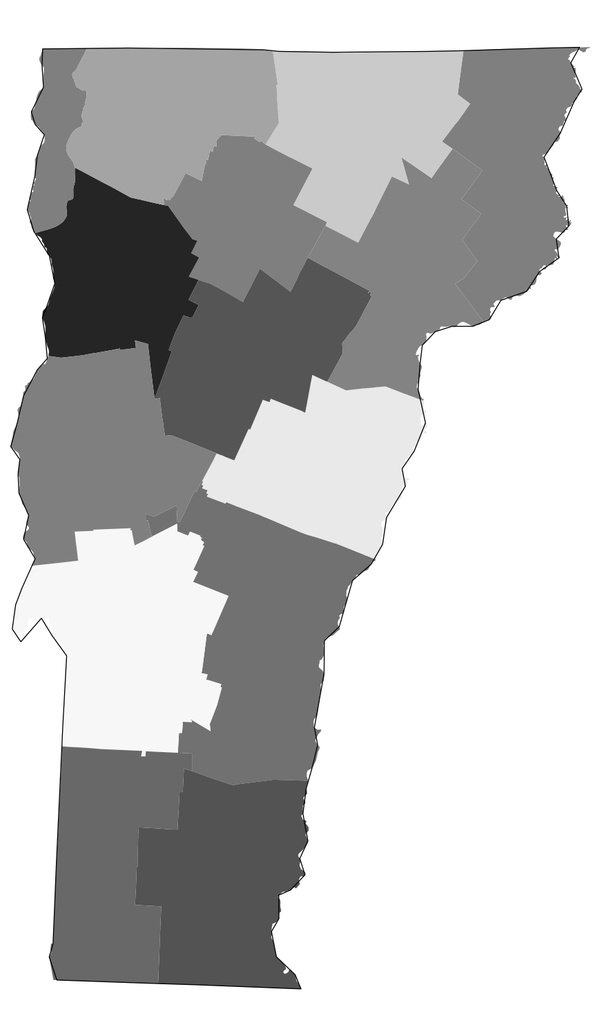
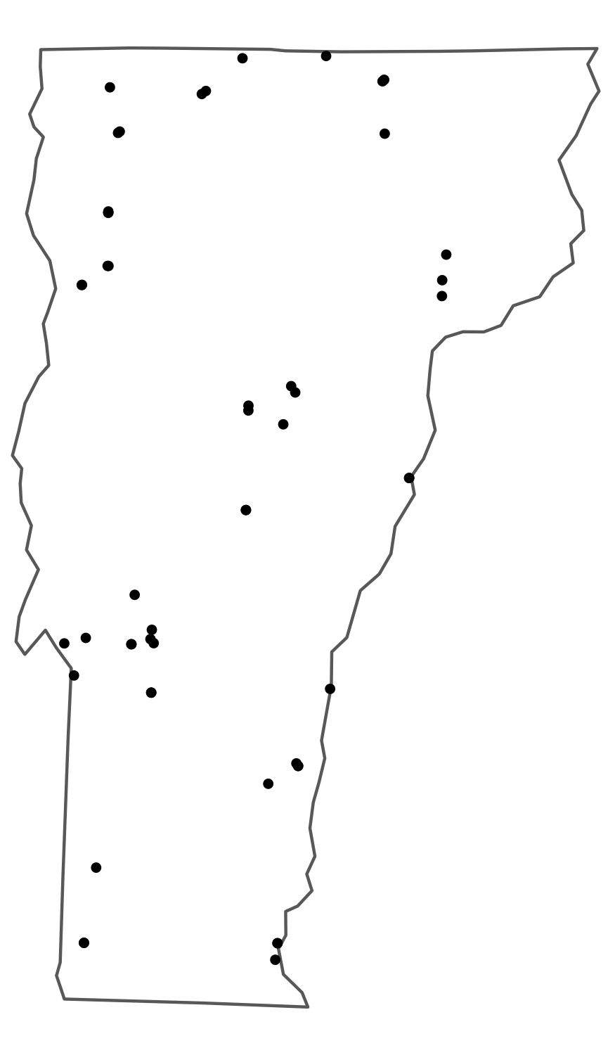
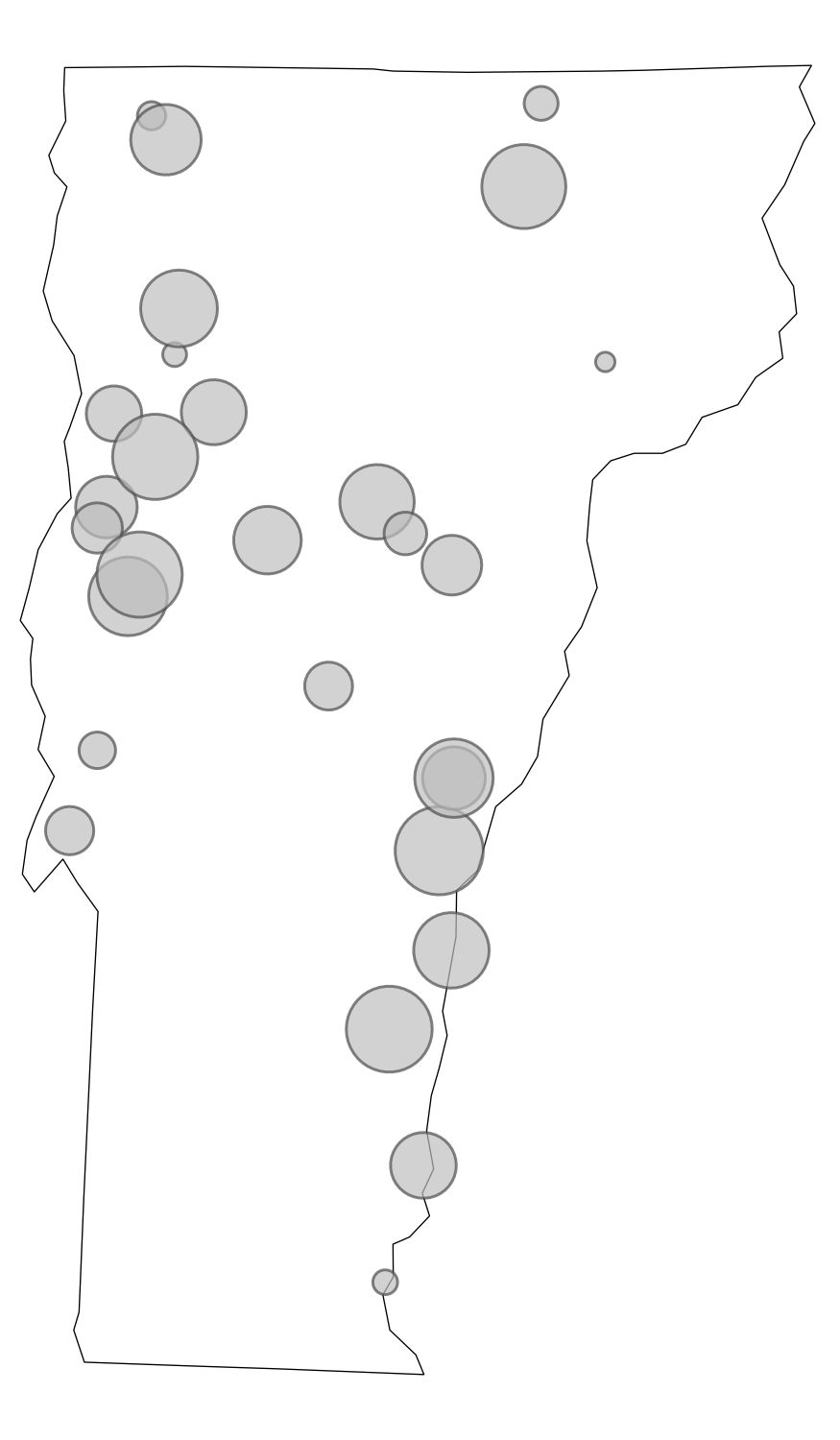
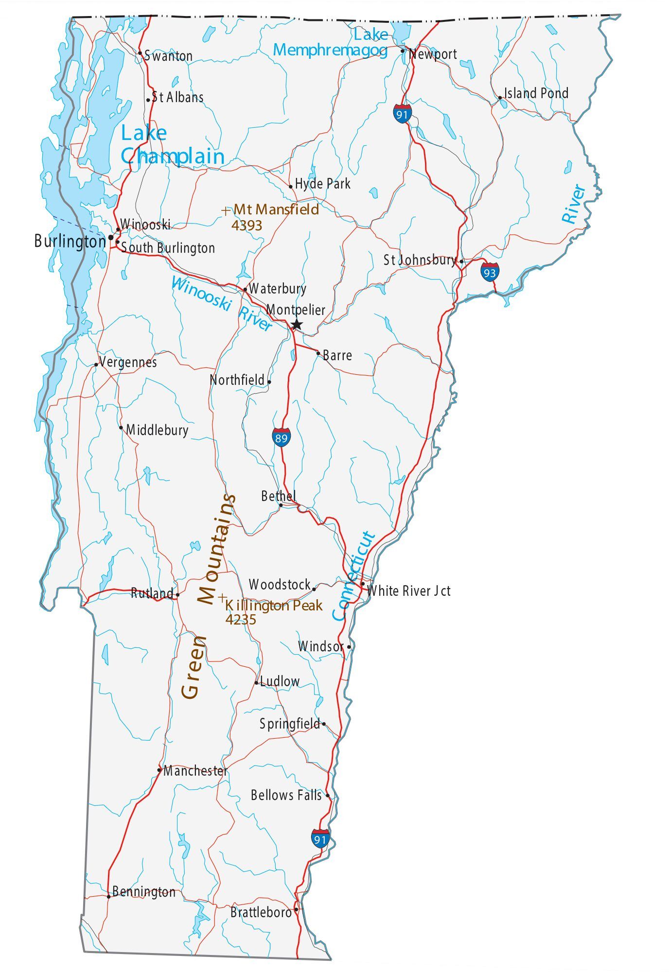
Choropleth: areas shaded by value

Dot map: one dot per unit

Proportional symbol: symbol size = quantity

Reference: orientation / context

Part 2: Mapping in ggplot2

Getting Boundary Data

• TIGER/Line files: the Census Bureau’s authoritative geographic boundary dataset, covering states, counties, tracts, roads, water features, and more
• tigris: an R package that downloads TIGER/Line files directly from the Census API and returns them as sf objects, ready to map

states_sf <- states(cb = TRUE, resolution = "20m") %>%
  filter(!STUSPS %in% c("AK", "HI", "PR", "VI", "GU", "AS", "MP"))

counties_sf <- counties(cb = TRUE, resolution = "20m") %>%
  filter(!STATEFP %in% c("02", "15", "72", "78", "66", "60", "69"))

• cb = TRUE: simplified cartographic boundary (better for maps)
• resolution = "20m": 1:20,000,000 scale (right for national maps)
• The filter removes Alaska, Hawaii, and territories

tigris has many other geographies too: tracts, block groups, places, school districts, congressional districts, ZIP codes, roads, water features. All come back as sf objects ready to use.

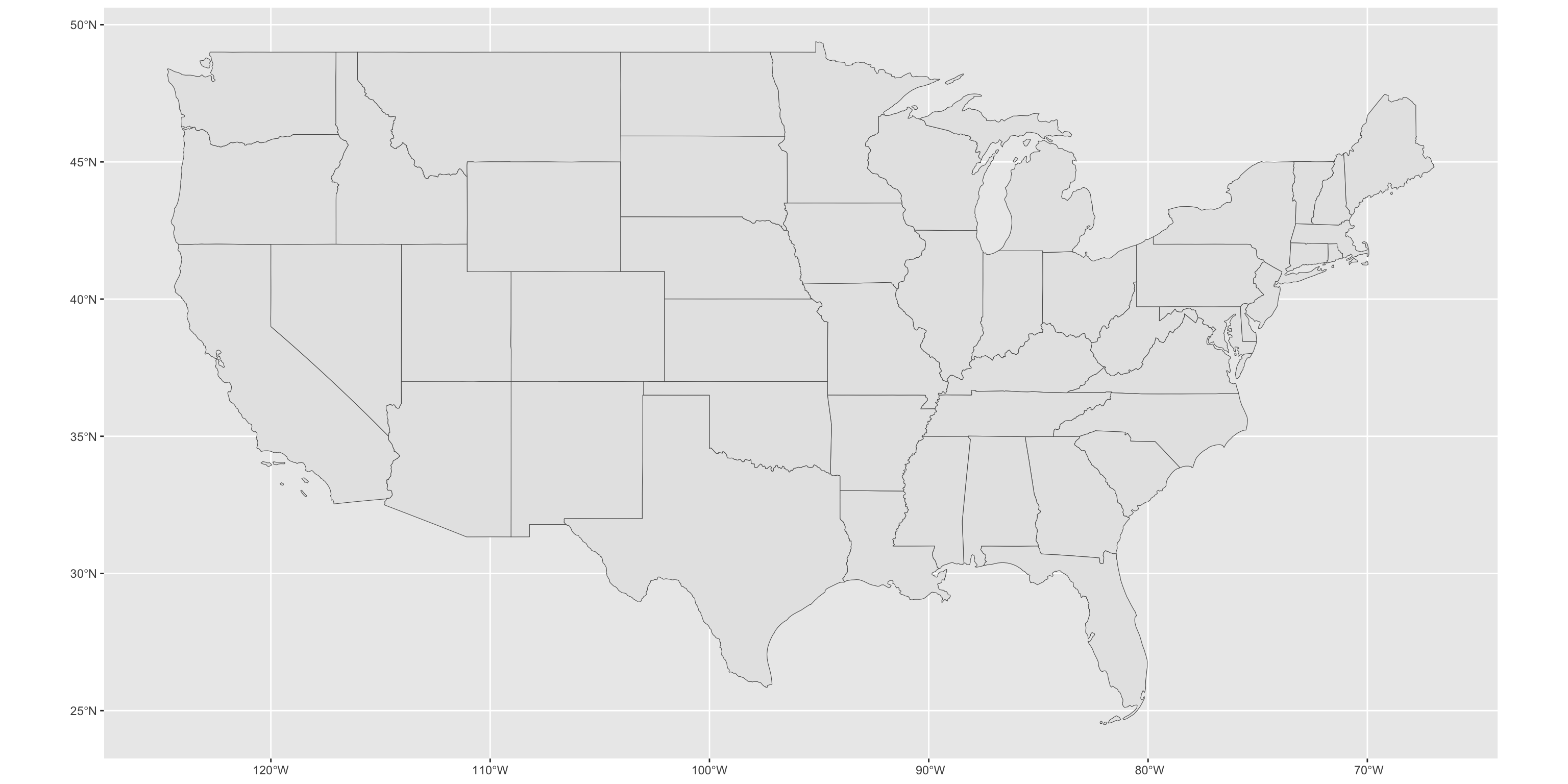
Your First Map

ggplot(states_sf) +
  geom_sf()

geom_sf() reads the geometry column and draws the shapes. But it looks flat and weird – let’s fix that.

Your First Map

Applying a Projection

ggplot(states_sf) +
  geom_sf() +
  coord_sf(crs = 5070)

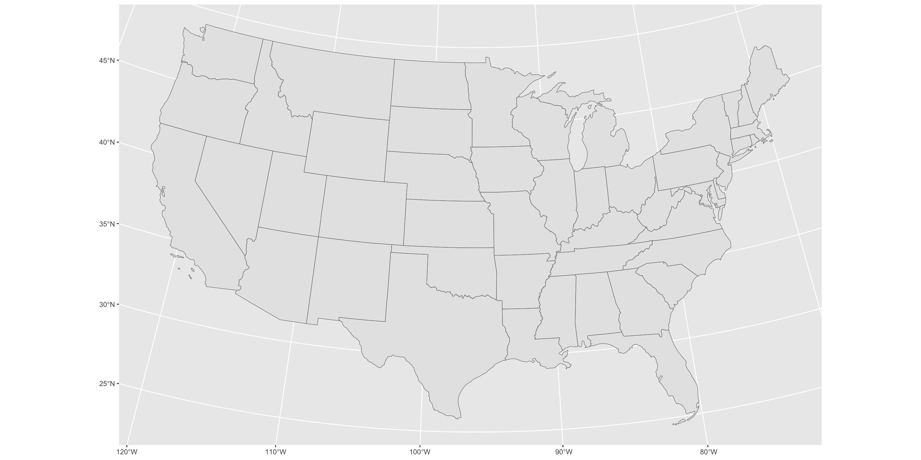
coord_sf() reprojects the visualization without modifying your data. This single line is the most impactful improvement you can make to a US national map.

Applying a Projection

Styling

ggplot(states_sf) +
  geom_sf(fill = "dodgerblue", color = "white", linewidth = 0.3) +
  coord_sf(crs = 5070) +
  theme_void()

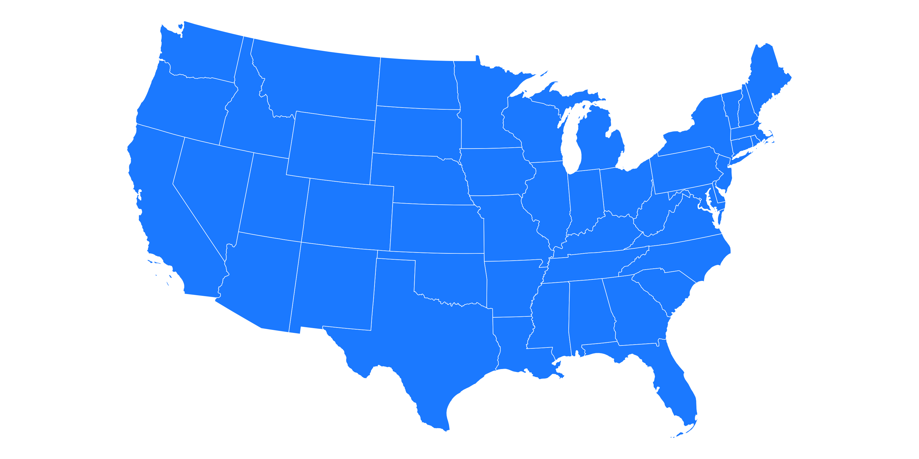
theme_void() removes axes, gridlines, and background – almost always the right choice for a finished map.

Styling

Real Data: LACE

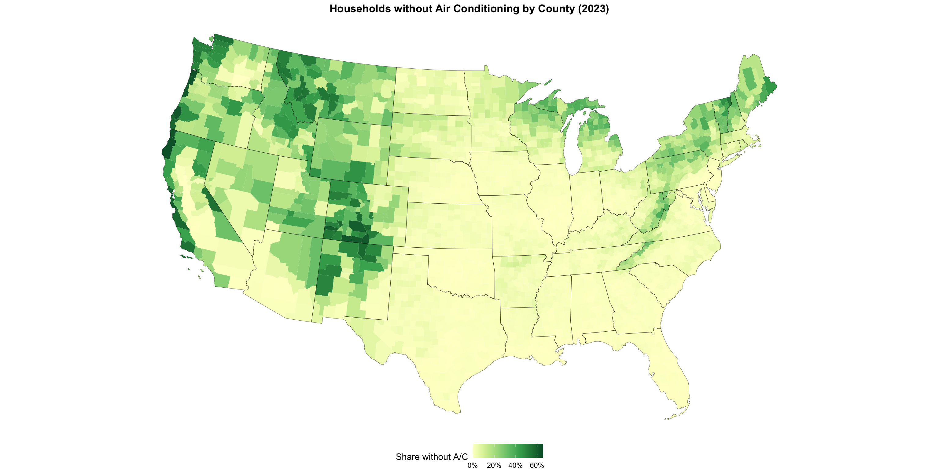
New from the Census Bureau: county-level estimates of households without air conditioning.

lace <- read_csv("https://www2.census.gov/programs-surveys/demo/datasets/lace/2023/LACE_23_County.csv") %>%
  mutate(GEOID = paste0(STATE, COUNTY))

lace_map <- counties_sf %>%
  left_join(lace, by = "GEOID")

This is the standard workflow: get boundaries from tigris, join your data on GEOID, map it.

GEOID is the 5-character FIPS code: 2-digit state + 3-digit county, always zero-padded. This is the universal join key for any Census-derived county data.

Building the Map Incrementally

ggplot(lace_map) +
  geom_sf(aes(fill = NO_AC_PE/100), color = NA) +
  geom_sf(data = states_sf, fill = NA, color = "black", linewidth = 0.1) +
  coord_sf(crs = 5070) +
  scale_fill_distiller(
    palette = "YlGn", direction = 1,
    labels = percent, name = "Share without A/C"
  ) +
  theme_void() +
  theme(legend.position = "bottom",
        plot.title = element_text(face = "bold", hjust = .5)) +
  labs(title = "Households without Air Conditioning by County (2023)")

[Live demo.] In demo_script.R, start with most of these arguments commented out. Uncomment one at a time so the audience can see what each piece contributes to the finished map.

Building the Map Incrementally

Color Scale Options

# Sequential (one hue, light to dark)
scale_fill_distiller(palette = "YlGn", direction = 1)
scale_fill_viridis_c(option = "rocket")

# Diverging (two hues, use when 0 means something)
scale_fill_distiller(palette = "RdBu", direction = 1)

# Right-skewed data: log-transform the scale
scale_fill_viridis_c(trans = "log10", labels = scales::comma)

Avoid rainbow palettes (rainbow(), jet). They are not perceptually uniform and create false visual boundaries in your data.

• ColorBrewer (colorbrewer2.org) — designed by cartographer Cynthia Brewer, it provides rigorously tested sequential, diverging, and qualitative palettes optimized for maps. No need to reinvent the wheel; the cartographers already laid the groundwork.

Part 3: Census and NASS Data

tidycensus

tidycensus pulls Census Bureau data directly into R, with geometry attached if you want it.

# one-time setup -- free key at api.census.gov/data/key_signup.html
census_api_key("YOUR_KEY_HERE", install = TRUE)

Covers: Decennial Census, ACS 1-year and 5-year, and more

ACS data is estimated, not a headcount. The smaller the geography, the larger the margin of error. A block group SNAP estimate has a much wider confidence interval than a county-level estimate.

Finding Variables

v22 <- load_variables(2022, "acs5", cache = TRUE)

v22 %>%
  filter(str_detect(label, regex("snap|food stamp", ignore_case = TRUE))) %>%
  select(name, label, concept)

# A tibble: 162 × 3
   name       label                                                      concept
   <chr>      <chr>                                                      <chr>  
 1 B09010_002 Estimate!!Total:!!Living in household with Supplemental S… Receip…
 2 B09010_003 Estimate!!Total:!!Living in household with Supplemental S… Receip…
 3 B09010_004 Estimate!!Total:!!Living in household with Supplemental S… Receip…
 4 B09010_005 Estimate!!Total:!!Living in household with Supplemental S… Receip…
 5 B09010_006 Estimate!!Total:!!Living in household with Supplemental S… Receip…
 6 B09010_007 Estimate!!Total:!!Living in household with Supplemental S… Receip…
 7 B09010_008 Estimate!!Total:!!Living in household with no Supplementa… Receip…
 8 B09010_009 Estimate!!Total:!!Living in household with no Supplementa… Receip…
 9 B09010_010 Estimate!!Total:!!Living in household with no Supplementa… Receip…
10 B09010_011 Estimate!!Total:!!Living in household with no Supplementa… Receip…
# ℹ 152 more rows

There are ~27,000 ACS 5-year variables. load_variables() + str_detect() is how you find what you need.

Pulling SNAP Data with Geometry

snap_households <- get_acs(
  geography = "county",
  variables = c(snap  = "B22003_002",
                total = "B22003_001"),
  year      = 2022,
  geometry  = TRUE
) %>%
  select(GEOID, NAME, variable, estimate) %>%
  pivot_wider(names_from = variable, values_from = estimate) %>%
  mutate(snap_pct = snap / total) %>%
  filter(!str_starts(GEOID, "02|15|72"))

geometry = TRUE is the killer feature: one call returns data and boundaries together.

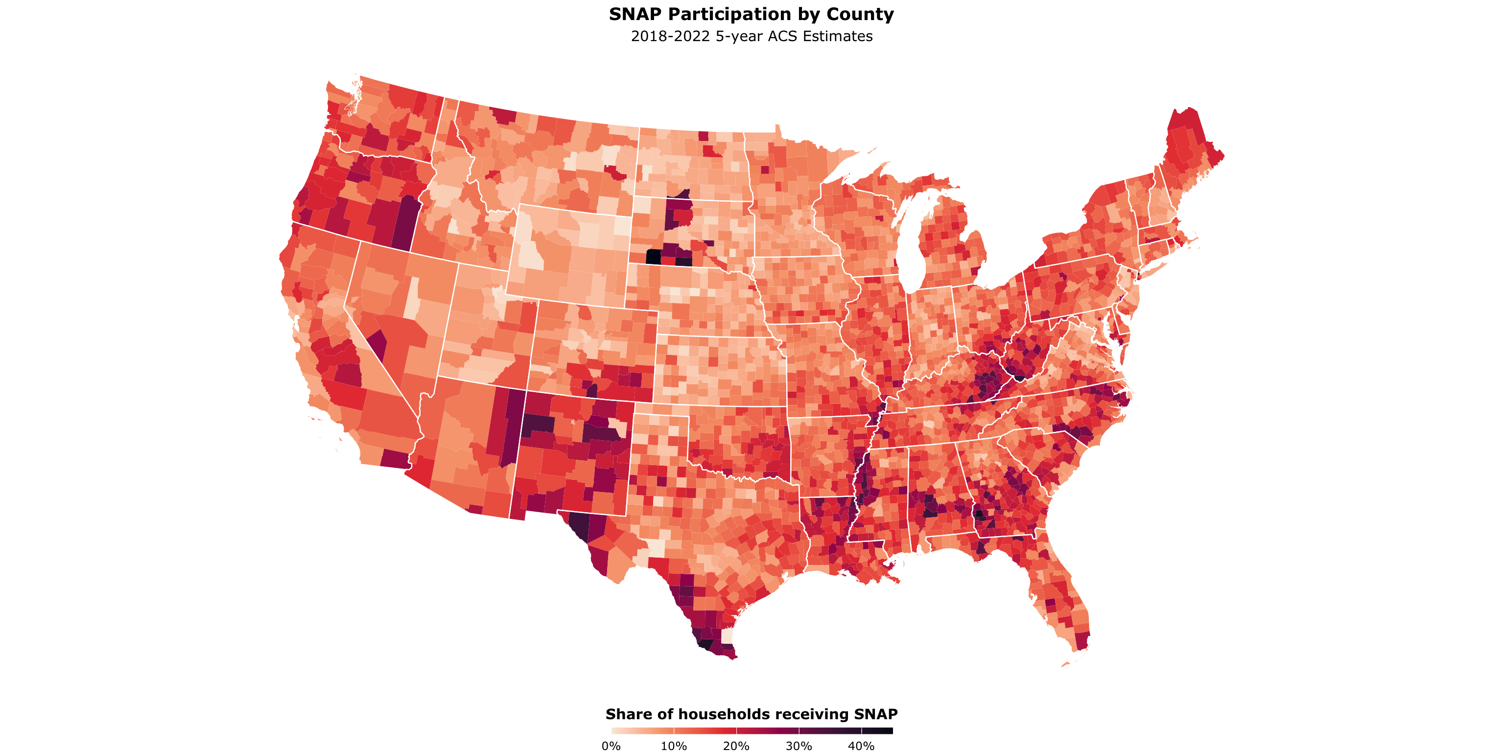
SNAP Participation by County

ggplot(snap_households) +
  geom_sf(aes(fill = snap_pct), color = NA) +
  geom_sf(data = states_sf, fill = NA, color = "white", linewidth = 0.4) +
  coord_sf(crs = 5070) +
  scale_fill_viridis_c(
    name = "Share of households receiving SNAP",
    labels = percent_format(accuracy = 1),
    option = "rocket", 
    direction = -1
  ) +
  theme_void(base_family = "Verdana") +
  theme(legend.position = "bottom",
        legend.title = element_text(face = "bold", hjust = .5),
        plot.title = element_text(face = "bold", hjust = .5),
        plot.subtitle = element_text(hjust = .5)) +
  guides(fill = guide_colourbar(barheight = 0.35, barwidth = 15, title.position = "top")) +
  labs(title = "SNAP Participation by County",
       subtitle = "2018-2022 5-year ACS Estimates")

SNAP Participation by County

Going Smaller: Census Tracts

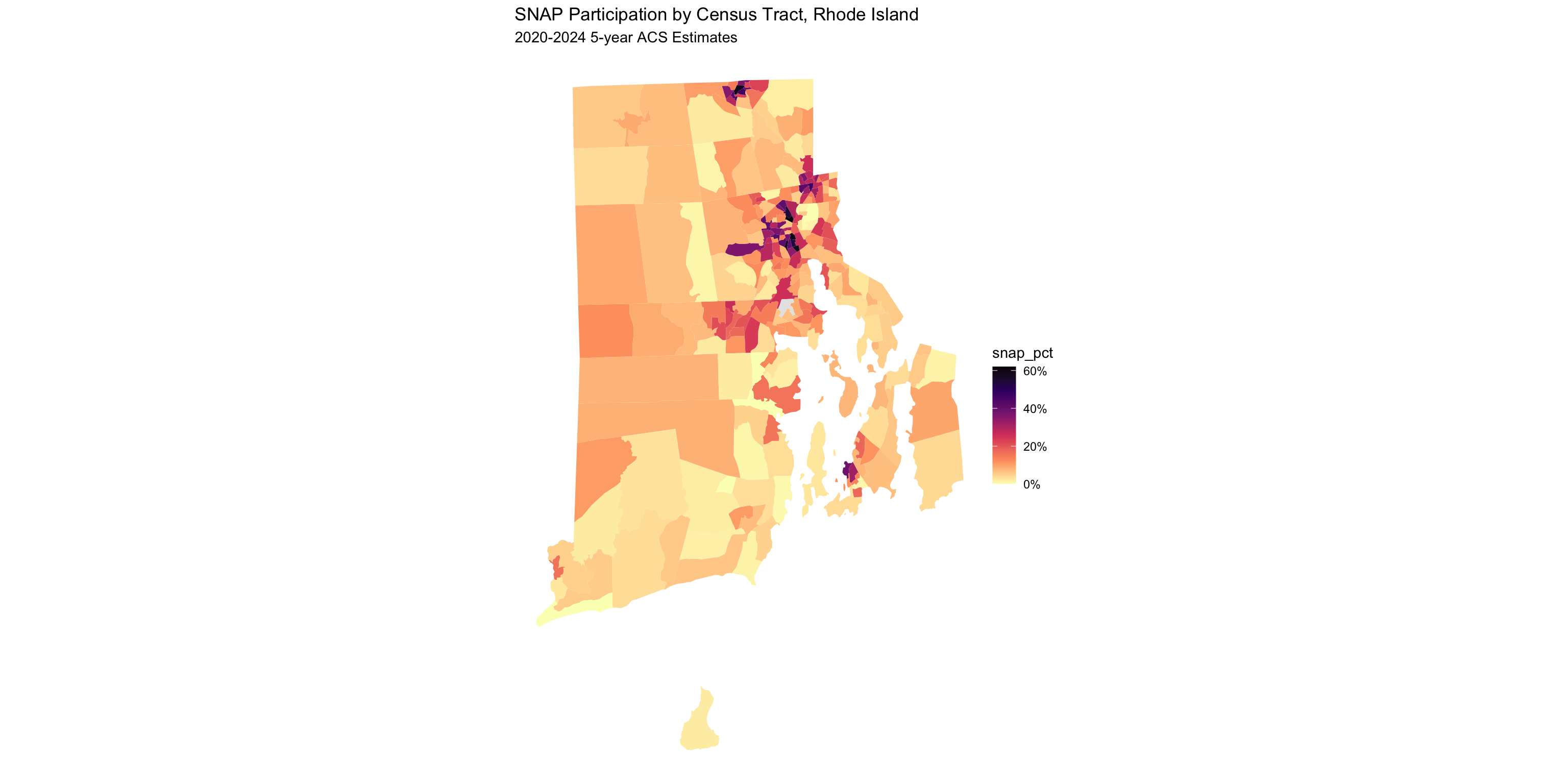
Change geography = "county" to geography = "tract" and add a state argument:

get_acs(
  geography = "tract", state = "RI",
  variables = c(snap = "B22003_002", total = "B22003_001"),
  year = 2024, geometry = TRUE
) %>%
  select(GEOID, NAME, variable, estimate) %>%
  pivot_wider(names_from = variable, values_from = estimate) %>%
  mutate(snap_pct = snap / total) %>%
  ggplot() +
  geom_sf(aes(fill = snap_pct), color = NA) +
  scale_fill_viridis_c(option = "A", direction = -1,
                       labels = percent_format(accuracy = 1),
                       na.value = "grey90") +
  theme_void() +
  labs(title = "SNAP Participation by Census Tract, Rhode Island",
       subtitle = "2020-2024 5-year ACS Estimates")

Everything is the same except geography and state. tidycensus supports county, tract, block group, place, ZCTA, and more.

Going Smaller: Census Tracts

NASS QuickStats: rnassqs

NASS QuickStats is USDA’s public database: crops, livestock, farm economics, farm counts, and more.

# one-time setup per session -- free key at quickstats.nass.usda.gov/api
nassqs_auth("YOUR_API_KEY")

Tip: prototype at quickstats.nass.usda.gov first to get exact parameter names and verify record counts before calling the API.

Querying NASS: Corn and Soybeans

corn_acres <- nassqs(
  commodity_desc = "CORN", short_desc = "CORN - ACRES PLANTED",
  domain_desc = "TOTAL", agg_level_desc = "COUNTY", year = 2015
) %>%
  mutate(GEOID = paste0(state_fips_code, county_code)) %>%
  select(GEOID, year, corn_acres_planted = Value)

soybean_acres <- nassqs(
  commodity_desc = "SOYBEANS", short_desc = "SOYBEANS - ACRES PLANTED",
  domain_desc = "TOTAL", agg_level_desc = "COUNTY", year = 2015
) %>%
  mutate(GEOID = paste0(state_fips_code, county_code)) %>%
  select(GEOID, year, soybean_acres_planted = Value)

corn_acres_sf    <- left_join(counties_sf, corn_acres)
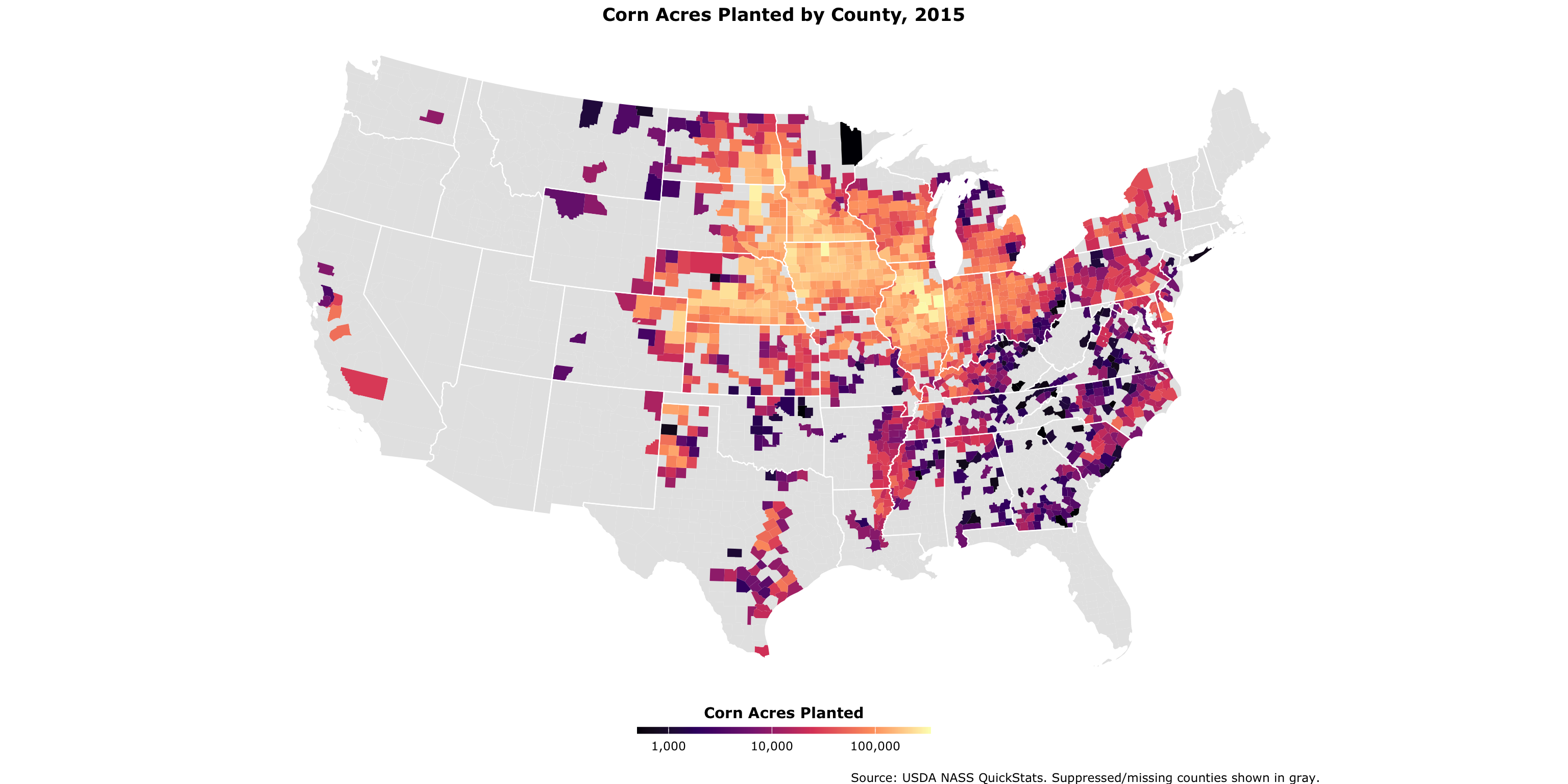
soybean_acres_sf <- left_join(counties_sf, soybean_acres)

Corn Acres Planted, 2015

ggplot(corn_acres_sf) +
  geom_sf(aes(fill = corn_acres_planted), color = NA) +
  geom_sf(data = states_sf, fill = NA, color = "white", linewidth = 0.4) +
  coord_sf(crs = 5070) +
  scale_fill_viridis_c(option = "A", name = "Corn Acres Planted",
                       labels = comma_format(), trans = "log10", na.value = "gray90") +
  theme_void(base_family = "Verdana") +
  theme(legend.position = "bottom",
        legend.title = element_text(face = "bold", hjust = .5),
        plot.title = element_text(face = "bold", hjust = .5)) +
  guides(fill = guide_colourbar(barheight = 0.35, barwidth = 15, title.position = "top")) +
  labs(title = "Corn Acres Planted by County, 2015",
       caption = "\nSource: USDA NASS QuickStats. Suppressed/missing counties shown in gray.")

Corn Acres Planted, 2015

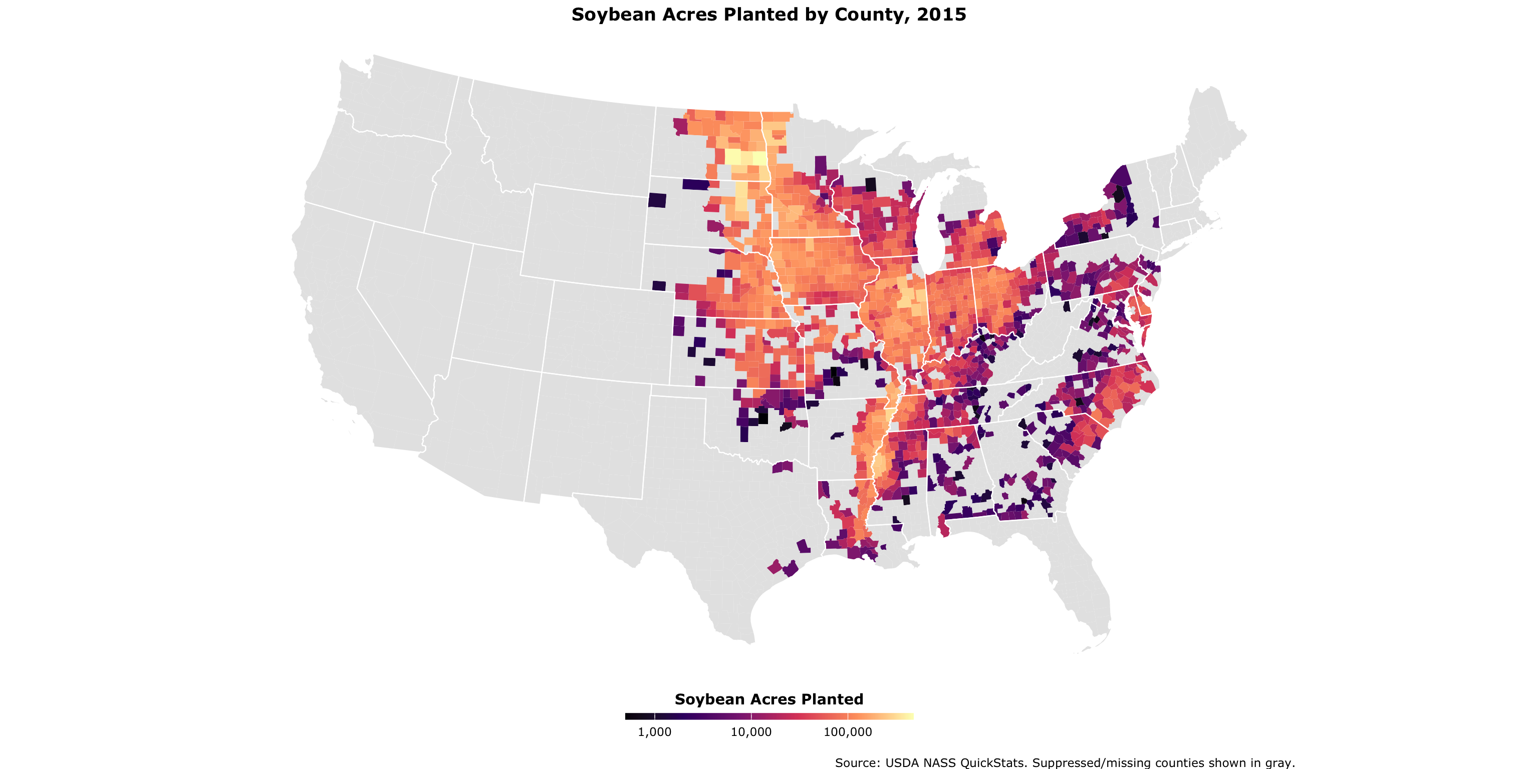
Soybean Acres Planted, 2015

ggplot(soybean_acres_sf) +
  geom_sf(aes(fill = soybean_acres_planted), color = NA) +
  geom_sf(data = states_sf, fill = NA, color = "white", linewidth = 0.4) +
  coord_sf(crs = 5070) +
  scale_fill_viridis_c(option = "A", name = "Soybean Acres Planted",
                       labels = comma_format(), trans = "log10", na.value = "gray90") +
  theme_void(base_family = "Verdana") +
  theme(legend.position = "bottom",
        legend.title = element_text(face = "bold", hjust = .5),
        plot.title = element_text(face = "bold", hjust = .5)) +
  guides(fill = guide_colourbar(barheight = 0.35, barwidth = 15, title.position = "top")) +
  labs(title = "Soybean Acres Planted by County, 2015",
       caption = "\nSource: USDA NASS QuickStats. Suppressed/missing counties shown in gray.")

Soybean Acres Planted, 2015

Finding Better Breaks: Jenks

Right-skewed ag data looks like one color with a linear scale. Jenks natural breaks fix that.

corn_vals <- as.numeric(str_remove_all(corn_acres_sf$corn_acres_planted, ","))
soy_vals  <- as.numeric(str_remove_all(soybean_acres_sf$soybean_acres_planted, ","))
combined  <- c(corn_vals, soy_vals)

brks <- classIntervals(
  combined[!is.na(combined) & combined > 0], n = 5, style = "jenks"
)$brks %>% round(-3)

pal <- brewer.pal(length(brks), "YlGn")

Using the combined distribution ensures both maps share the same color scale.

Comparing Maps with compare()

left_map <- maplibre(bounds = states_sf, style = carto_style("voyager")) %>%
  add_fill_layer(id = "corn_acres", source = corn_acres_sf,
    fill_color = interpolate(column = "corn_acres_planted",
                             values = brks, stops = pal, na_color = "lightgrey"),
    fill_opacity = 0.9, tooltip = "corn_acres_planted") %>%
  add_line_layer(id = "states", source = states_sf, line_width = .1) %>%
  add_continuous_legend("Corn Acres Planted, 2015",
    values = brks, colors = pal, position = "top-left")

right_map <- maplibre(bounds = states_sf, style = carto_style("voyager")) %>%
  add_fill_layer(id = "soybean_acres", source = soybean_acres_sf,
    fill_color = interpolate(column = "soybean_acres_planted",
                             values = brks, stops = pal, na_color = "lightgrey"),
    fill_opacity = 0.9, tooltip = "soybean_acres_planted") %>%
  add_line_layer(id = "states", source = states_sf, line_width = .1) %>%
  add_continuous_legend("Soybean Acres Planted, 2015",
    values = brks, colors = pal, position = "top-left")

compare(left_map, right_map, height = "900px")

Comparing Maps with compare()

Part 4: Point Data and GIS

From Table to Map

Any table with latitude and longitude columns can become a spatial dataset.

usda_inspection_estabs <- read_csv("https://andrewvanleuven.github.io/aaea_webinar/data/MPI_Directory_by_Establishment_Number.csv")
glimpse(usda_inspection_estabs)

Rows: 7,185
Columns: 21
$ establishment_id     <dbl> 126740, 195, 126734, 126639, 6164012, 8204, 8193,…
$ establishment_number <chr> "G1016", "G1028", "G1105", "G1126A+V1126A", "G112…
$ establishment_name   <chr> "M.G. Waldbaum Company", "Papetti's Hygrade Egg P…
$ duns_number          <chr> "18076351", "7266158", NA, "72983554", "15396242"…
$ street               <chr> "430 Railroad Avenue", "One Papetti Plaza", "375 …
$ city                 <chr> "Gaylord", "Elizabeth", "Blackshear", "Spanish Fo…
$ state                <chr> "MN", "NJ", "GA", "UT", "UT", "IL", "NJ", "IA", "…
$ zip                  <chr> "55334", "7206", "31516", "84660", "84660", "6283…
$ phone                <chr> "(507) 237-4600", "(908) 282-7900", "(912) 449-57…
$ grant_date           <chr> "1/28/2026", "12/5/2019", "9/22/2021", "1/28/2022…
$ activities           <chr> "Egg Product", "Egg Product", "Egg Product", "Cer…
$ dbas                 <chr> "Michael Foods Inc.", NA, NA, NA, "Muscle Egg", N…
$ district             <dbl> 25, 80, 85, 15, 15, 50, 80, 25, 25, 50, 60, 15, 8…
$ circuit              <chr> "2507", "8020", "8509", "1532", "1532", "5007", "…
$ size                 <chr> "N / A", "Small", "Small", "Small", "Very Small",…
$ latitude             <dbl> 44.55444, 40.65799, 31.30408, 40.11510, 40.11414,…
$ longitude            <dbl> -94.20699, -74.18885, -82.23269, -111.73739, -111…
$ county               <chr> "Sibley County", "Union County", "Pierce County",…
$ fips_code            <dbl> 27143, 34039, 13229, 49049, 49049, 17051, 34039, …
$ LatestMPIActiveDate  <chr> "6/1/2026", "6/1/2026", "6/1/2026", "6/1/2026", "…
$ est_status           <lgl> NA, NA, NA, NA, NA, NA, NA, NA, NA, NA, NA, NA, N…

Source: USDA FSIS Meat, Poultry & Egg Product Inspection Directory.

st_as_sf(): Adding Geometry

usda_inspection_estabs_sf <- usda_inspection_estabs %>%
  mutate(across(where(is.character), ~iconv(., to = "UTF-8", sub = ""))) %>%
  st_as_sf(coords = c("longitude", "latitude"), crs = 4326, remove = FALSE) %>%
  st_transform(crs = 5070)

lower48_usda <- st_intersection(
  usda_inspection_estabs_sf,
  st_transform(states_sf, 5070)
) %>%
  filter(size %in% c("Large", "Small", "Very Small"))

st_as_sf() turns lat/lon columns into a geometry column. After that, it’s a normal sf object.

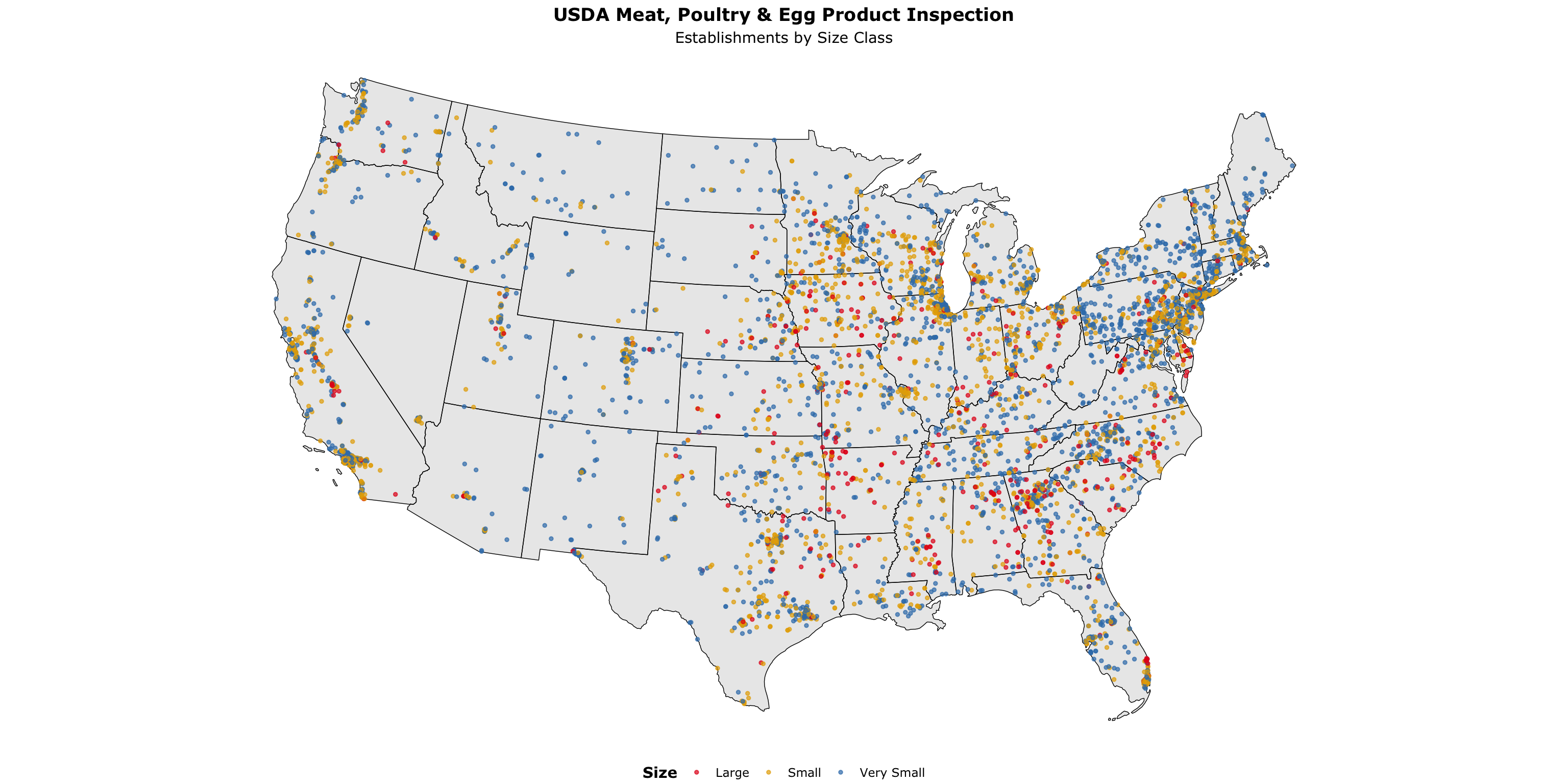
USDA Inspection Establishments

ggplot() +
  geom_sf(data = st_transform(states_sf, 5070), color = "black", linewidth = .25) +
  geom_sf(data = lower48_usda, aes(color = size), size = 1, alpha = .7) +
  scale_color_manual(values = c("#e41a1c", "#e6ab02", "#377eb8"), name = "Size") +
  theme_void(base_family = "Verdana") +
  theme(legend.position = "bottom",
        legend.title = element_text(face = "bold", hjust = .5),
        plot.subtitle = element_text(hjust = .5),
        plot.title = element_text(face = "bold", hjust = .5)) +
  labs(title = "USDA Meat, Poultry & Egg Product Inspection",
       subtitle = "Establishments by Size Class")

USDA Inspection Establishments

Categorical Point Maps with mapgl

gas_stations <- read_csv("https://andrewvanleuven.github.io/aaea_webinar/data/gas_stations.csv") %>%
  st_as_sf(wkt = "geometry_wkt", crs = 4326) %>%
  st_transform(crs = 5070)

maplibre(style = carto_style("positron"), bounds = states_sf) %>%
  add_circle_layer(
    id = "poi-gas", source = gas_stations,
    circle_color = match_expr("name",
      values = c("Casey's General Store", "Cenex", "Kwik Trip/Kwik Star"),
      stops  = c("#F3D317", "#8a0000", "#0300ad")),
    circle_radius = 4, circle_stroke_color = "#ffffff",
    circle_stroke_width = .4, circle_opacity = 0.7, tooltip = "city_name"
  ) %>%
  add_line_layer(id = "states", source = states_sf, line_width = .1) %>%
  add_categorical_legend(
    legend_title = "Midwest Gas Station Chains",
    values = c("Casey's General Store", "Cenex", "Kwik Trip/Kwik Star"),
    colors = c("#F3D317", "#8a0000", "#0300ad"),
    patch_shape = "circle", position = "bottom-left",
    layer_id = "poi-gas", interactive = TRUE
  )

Categorical Point Maps with mapgl

Categorical Point Maps with mapgl

dollar_stores <- read_csv("https://andrewvanleuven.github.io/aaea_webinar/data/dollar_stores.csv") %>%
  st_as_sf(wkt = "geometry_wkt", crs = 4326) %>%
  st_transform(crs = 5070) %>%
  mutate(tooltip = glue("<b>{name}</b><br>{city_name}"))

maplibre(style = carto_style("positron"), bounds = states_sf) %>%
  add_circle_layer(
    id           = "poi-dollar-store",
    source       = dollar_stores,
    circle_color = match_expr(
      "name",
      values = c("Dollar General", "Dollar Tree", "Family Dollar"),
      stops  = c("#fff200", "#00954C", "#E81F11")
    ),
    circle_radius       = 4,
    circle_stroke_color = "black",
    circle_stroke_width = .4,
    circle_opacity      = 0.7,
    tooltip             = "tooltip"
  ) %>%
  add_categorical_legend(
    legend_title = "Dollar Store Establishments",
    values       = c("Dollar General", "Dollar Tree", "Family Dollar"),
    colors       = c("#fff200", "#00954C", "#E81F11"),
    patch_shape  = "circle",
    position     = "bottom-left",
    layer_id     = "poi-dollar-store",
    interactive  = TRUE
  )

Categorical Point Maps with mapgl

st_intersection: Points in Polygons

dollar_stores <- read_csv("https://andrewvanleuven.github.io/aaea_webinar/data/dollar_stores.csv") %>%
  st_as_sf(wkt = "geometry_wkt", crs = 4326) %>%
  st_transform(crs = 5070) %>%
  mutate(tooltip = glue("<b>{name}</b><br>{city_name}"))

county_pop_2020 <- get_decennial(geography = "county", variables = "P1_001N",
  year = 2020, geometry = TRUE) %>%
  st_transform(5070) %>%
  filter(!str_starts(GEOID, "02|15|72")) %>%
  select(cty_fips = GEOID, pop20 = value)

dollar_store_sf <- st_intersection(dollar_stores, county_pop_2020) %>%
  st_drop_geometry() %>%
  summarize(dollar_stores = n(), pop_2020 = first(pop20), .by = cty_fips) %>%
  replace_na(list(dollar_stores = 0)) %>%
  mutate(dollar_stores_per_capita = dollar_stores / pop_2020) %>%
  right_join(county_pop_2020, by = "cty_fips") %>%
  st_as_sf()

Raw Counts vs Per Capita

p1 <- ggplot() +
  geom_sf(data = dollar_store_sf, aes(fill = dollar_stores), color = NA) +
  geom_sf(data = states_sf, color = "white", linewidth = .35, fill = NA) +
  scale_fill_viridis_c(option = "mako", name = "# Establishments",
                       trans = "log10", direction = -1, na.value = "gray90") +
  theme_void() + theme(legend.position = "bottom") +
  labs(title = "Raw counts")

p2 <- ggplot() +
  geom_sf(data = dollar_store_sf,
          aes(fill = dollar_stores_per_capita * 10000), color = NA) +
  geom_sf(data = states_sf, color = "black", linewidth = .15, fill = NA) +
  scale_fill_distiller(palette = "YlOrBr", name = "Per 10,000 residents",
                       direction = 1, na.value = "white") +
  theme_void() + theme(legend.position = "bottom") +
  labs(title = "Per capita")

library(patchwork)
p1 + p2

Raw counts favor dense, populous counties. Per-capita rates let you compare across places of very different sizes. Always normalize for a choropleth unless you’re specifically making a point about total volume.

Raw Counts vs Per Capita

Buffer Analysis: st_buffer

iowa_dollar_stores <- dollar_stores %>%
  filter(state == "IA") %>%
  st_transform(6463) %>%
  st_buffer(10 * 5280) %>%
  st_transform(4326)

maplibre(bounds = filter(states_sf, STUSPS == "IA"),
         style = carto_style("positron")) %>%
  add_fill_layer(
    id = "buffers", source = iowa_dollar_stores,
    fill_color = "#202020", fill_opacity = 0.4
  )

st_buffer() creates a polygon a fixed distance around each point. CRS 6463 (Iowa State Plane) uses U.S. feet, so 1 mile = 5,280 feet.

Buffer Analysis: st_buffer

From Dense Points to Heatmap

iowa_pts <- dollar_stores %>%
  filter(state == "IA") %>%
  st_transform(4326) %>%
  st_jitter(factor = 0.0001)

maplibre(style = carto_style("positron"),
         bounds = filter(states_sf, STUSPS == "IA")) %>%
  add_circle_layer(
    id = "poi-dollar-store", source = iowa_pts,
    circle_color = "red", circle_stroke_color = "white", circle_stroke_width = 1
  ) %>%
  add_heatmap_layer(
    id = "heatmap", source = iowa_pts, heatmap_radius = 35,
    heatmap_color = interpolate(
      property = "heatmap-density", values = seq(0, 1, 0.2),
      stops = c("transparent", magma(5))
    )
  )

From Dense Points to Heatmap

More Things sf Can Do

st_distance()        # distance between features (in CRS units)
st_nearest_feature() # index of the nearest feature in another layer
st_centroid()        # geometric center of a polygon
st_area()            # area of a polygon (in CRS units)
st_union()           # merge / dissolve geometries into one
st_bbox()            # bounding box of a layer
st_crop()            # clip features to a rectangular extent
st_within()          # is feature A fully inside feature B?
st_touches()         # do features share a boundary?

sf cheat sheet: rstudio.github.io/cheatsheets/sf.pdf

More Examples of Spatial Data Visualization in R

More Examples of Spatial Data Visualization in R

More Examples of Spatial Data Visualization in R

More Examples of Spatial Data Visualization in R

Wrap Up

What We Covered

1. Mapping basics: vector vs. raster data, coordinate reference systems, map types
2. ggplot2 maps: tigris for boundaries, geom_sf(), projections, color scales, choropleth maps
3. Census and NASS data: tidycensus with geometry, SNAP participation maps, rnassqs for QuickStats, classification breaks, side-by-side map comparison
4. Point data and GIS operations: st_as_sf(), categorical styling, spatial joins, counts vs. rates, buffer analysis, heatmaps

Thank You

Andrew Van Leuven University of Vermont

andrew.vanleuven@uvm.edu

https://andrewvanleuven.com

Questions?

Thank the organizers (Zoë Plakias, Anne Byrne, and the challenge committee). Remind folks about the challenge deadline and the other two webinars (Jared Hutchins on data viz principles, Sid Bora on R data viz).